

A Complete Guide to Spherical Equivariant Graph Transformers
A 2.5-hour breakdown of spherical equivariant graph neural networks (EGNNs) and a deconstruction of the SE(3)-Transformer model.

Update: a technical version of this article is now published on arXiv! If you find this article helpful for your publications, please consider citing the published version below:
@article{tang2025complete,
  title={A Complete Guide to Spherical Equivariant Graph Transformers},
  author={Tang, Sophia},
  journal={arXiv preprint arXiv:2512.13927},
  year={2025}
}
Introduction
Over the past month, I’ve become obsessed with understanding the architecture behind the protein-prediction model, RoseTTAFold, which ultimately led me down a deep (but fascinating) rabbit hole of geometric graph neural networks (geometric GNNs).
The RosseTTAFold model leverages a three-path approach that incorporates multiple classes of input data (sequence MSA, 2D distance map, and 3D coordinates) to predict protein structure. Here, I will break down how to handle 3D geometric data for deep learning, which I find to be a beautiful example of how concepts from quantum physics, mathematics, biology, and computer science work together.
Generative protein structure prediction models like RoseTTAFold and AlphaFold have two primary modules: the sequence module that converts protein sequence data into a 3D representation of the protein, and a structure module where geometric GNNs come in. At a high level, geometric GNNs in the structure module function by:
Converting the initial 3D representation into a graph with nodes representing amino acids, arrays of feature data corresponding to each node, spatial coordinates describing a node’s relative location in 3D space, and edges containing information on pair-wise interactions between residues.
Computing updates for the feature embedding of each node from all connected nodes with an equivariant message-passing layer, which leverages learnable kernels that respect the spatial symmetries of the graph to transform the feature embeddings of adjacent nodes into a message used to update the feature embedding at the center node.
Aggregating messages from all adjacent nodes with a permutation-invariant and rotation-equivariant operator (e.g., mean or sum) that does not depend on the order in which the messages are aggregated and transforms equivariantly under rotation of the graph.
Updating the feature embedding of the center node using a combination of its input features (self-interaction) and the aggregated message from adjacent nodes (neighbor-to-center message-passing).
Performing the message-passing process for every node in the graph in parallel to generate an updated set of coordinates and displacement vectors between residues or atoms in the protein backbone (C-alpha atom, amine, and carboxyl groups).
Iteratively refining the graph based on the updated structure to minimize the loss function until convergence. The final graph represents the 3D protein structure with high spatial precision.
Not only are geometric GNNs useful for protein structure prediction, but they also have extensive applications in chemical property prediction, molecular dynamics simulation, and the generative design of biomolecules.
This article will focus on a specific type of geometric GNN called Spherical Equivariant GNNs (Spherical EGNNs), which are extremely useful in tasks dealing with geometric graph representations of objects with rotational symmetries, like molecules and proteins. Then, we will describe a specific spherical EGNN called the SE(3)-Transformer that incorporates the self-attention mechanism for molecular property prediction.
Underlying geometric GNNs are a lot of technically challenging concepts to grasp, involving quantum physics and mathematics, so this article aims to break down the fundamental concepts of spherical EGNNs intuitively and extend these concepts to deconstruct the Tensor Field Network and SE(3)-Transformer models. At the end of the article, I will discuss how these models can be applied for chemical property prediction on the QM9 dataset.
Preface
The majority of notation used in this article aligns with the convention used in the SE(3)-Transformers paper. In the original paper, specific indices distinguishing which kernels are unique and the extension to multiple channels of each feature type are omitted for brevity, but I included an expanded version in this article for completeness. Thus, the mathematical symbols denoting weights, kernels, vectors, and feature tensors have several sub- and superscripts that can refer to the following meanings:
in, out → input features and output features (after message-passing)
i → center node or destination node.
j → nodes in the neighborhood of node i with an outgoing edge pointing towards node i.
k → the type/degree of node features from the source or neighborhood nodes.
c_k → index of the type-k feature channel.
l → the type/degree of node features from the center node.
c_l → index of the type-l feature channel.
m_l, m_k, m → indices of the elements of the type-l, type-k, and type-J spherical tensors, which also correspond to magnetic quantum numbers corresponding to the angular momentum numbers l, k, and J
J → the intermediate feature types for spherical harmonics projections ranging from |k - l| to |k + l|.
ij → denotes an edge feature (displacement vector) or embedding stored in the edge (messages or key and value embeddings) from the neighborhood node j to the center node i.
lk→ denotes equivariant kernels that transform tensors from type-k to type-l features.
Q, K, V → denotes the kernels that transform features into query, key, and value embeddings, respectively.
mi → total input channels (or multiplicity) of degree di.
mo → total output channels of degree do.
Throughout the article, I have included code from the full PyTorch implementation of the SE(3)-Transformer on GitHub that I fully annotated and made slight modifications for clarity. I’ll be breaking down most of the classes found in the modules file on GitHub, but placing more emphasis on the mathematics and intuition surrounding the code, so I encourage you to refer to the full implementation to connect the snippets and intuition you gain from this article to the full functions and classes.
The code uses a Python library called Deep Graph Library (DGL) that allows the construction and handling of graph data. The library supports User-Defined Functions (UDFs) that enable users to construct novel functions that can be applied for message-passing across the entire graph (much of the code described here is encapsulated in a UDF). Here are some basic DGL notations that will be useful in interpreting the code throughout the article:
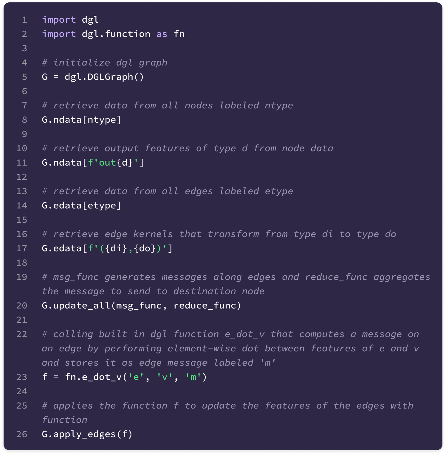
You can also find the documentation for the DGL library here.
In this article, we will be discussing geometric tensors (spherical tensors and Cartesian tensors) as well as working with the ‘tensor’ data structure in PyTorch, which refers to multidimensional arrays. To distinguish the two, I will use ‘tensor’ when referring to geometric tensors and ‘arrays’ when referring to the data structure.
When I state the shape of an array, I often omit the batch size (often the first dimension) used for smoother training and parallel computation, so the shape refers to the final dimensions of the tensor that are relevant to calculations.
Finally, since we will be discussing how attention works on geometric graphs, I highly recommend reading my previous article to get a foundational understanding of self-attention on sequence data before leveling up to three dimensions.
Preserving Rotational Equivariance
Understanding how to preserve rotational equivariance is the primary challenge of understanding geometric GNNs. Conventional deep learning models generate predictions based on learned features on a fixed reference frame but fail to detect those same features after transformations in space.
Rotational symmetries are rooted in all physical systems, especially on the molecular scale. Thus, constructing models that understand how interactions between nodes change under rotation is critical for tasks involving biomolecular systems.
Invariance and Equivariance
Invariance and equivariance are the cornerstones of geometric GNNs because they describe how convolutions or filters must be constructed to recognize patterns and generate predictions on a global reference frame where the graph can appear in any location or orientation in space but encode data that is the same or differing by a predictable transformation.
When a function produces the same output for a given input regardless of its orientation or position in space, it preserves invariance. A feature of a physical system can also be called invariant if it does not change with permutations or rotations (e.g., atomic number, bond type, number of protons). Only functions that preserve invariance should be applied to invariant features.
For instance, the potential energy of an isolated molecule in a vacuum is constant no matter its orientation or position in space; therefore, a function that calculates the potential energy given a molecule input should produce the same value no matter its position or orientation; in other words, it should preserve invariance.
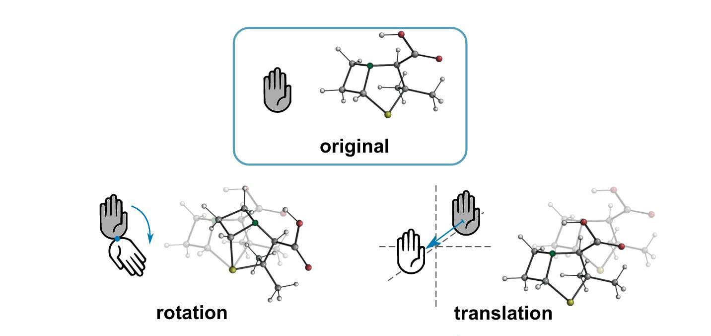
When a function produces a predictable transformation of the original output as a direct consequence of a transformation on the input (i.e. translation or rotation), it preserves equivariance.
A node feature is equivariant if it transforms predictably under transformations in the node’s position, and similarly, an edge feature is equivariant if it transforms predictably under transformations in either node it connects. Features on the node level of a geometric graph are often equivariant as they change with changes to the relative position and orientation of nodes, whereas system-level properties across the entire system are generally invariant. Only functions that preserve equivariance should be applied to equivariant features.
All chemical features represented by vectors (e.g. position, velocity, external forces on individual atoms) are equivariant, as they should transform with transformations in the input. In a molecule, changing the position of a negatively charged atom changes the direction of the attractive force between it and nearby charged atoms.
Preserving equivariance is crucial for modeling molecular systems, as their behavior is governed by conserved quantities of quantum mechanics, like angular momentum and energy, that follow strict sets of physical laws with inherent rotational symmetries.
Transformation equivariant models ensure that three-dimensional spatial transformations (i.e. translations in x, y, and z directions and rotations around any axis) of the input graph structure and features result in predictable transformations in the model’s output using functions (called kernels) that learn patterns across positional and feature data and applies them equivariantly across the entire graph. These functions are applied across the graph and are constructed to handle location and orientation-invariant or equivariant features without needing to be trained on rotated or translated data.
Similar to how a convolutional neural network (CNN) applies position-invariant filters to detect two-dimensional motifs regardless of their position in the input (i.e. image, heatmap), equivariant GNNs apply the same transformation-equivariant filters to detect motifs regardless of translations and rotations in 3D space.
Group Representations and Transformation Operators
A group in mathematics is defined as a set, denoted as G, of abstract actions (e.g. rotations and translations) and a binary operation ab for all a, b ∈ G that operates on the elements in the set such that the following conditions hold:
Closure — for all a, b ∈ G, the output of the binary operator is also in the set, ab ∈ G.
Associativity — for all a, b, c ∈ G, the following equation holds: (ab)c = a(bc)
Identity Element — every group has an identity element e that returns the element unchanged when applied to any element in the set with the binary operator. In other words, for all a ∈ G, ea = ae = a.
Inverse Element — for all a ∈ G, there exists an inverse of a (denoted as a⁻¹) in G such that aa⁻¹ = a⁻¹a = e (identity element). Note that a is also the inverse of a⁻¹.
A group representation converts the abstract elements of a group into a set of N x N invertible square matrices, denoted as GL(N). A group representation is generated via a group homomorphism ρ: G → GL(N) that takes a group as input and outputs a set of N x N matrices corresponding to each group element while preserving the function of the binary operator:
These representations can also be interpreted as injective transformation operators that act on N-dimensional vectors in a specific subspace, mapping the vector from one point in the subspace to another point in the same subspace. With the idea of group representations as transformation operators, we can define invariant and equivariant functions.
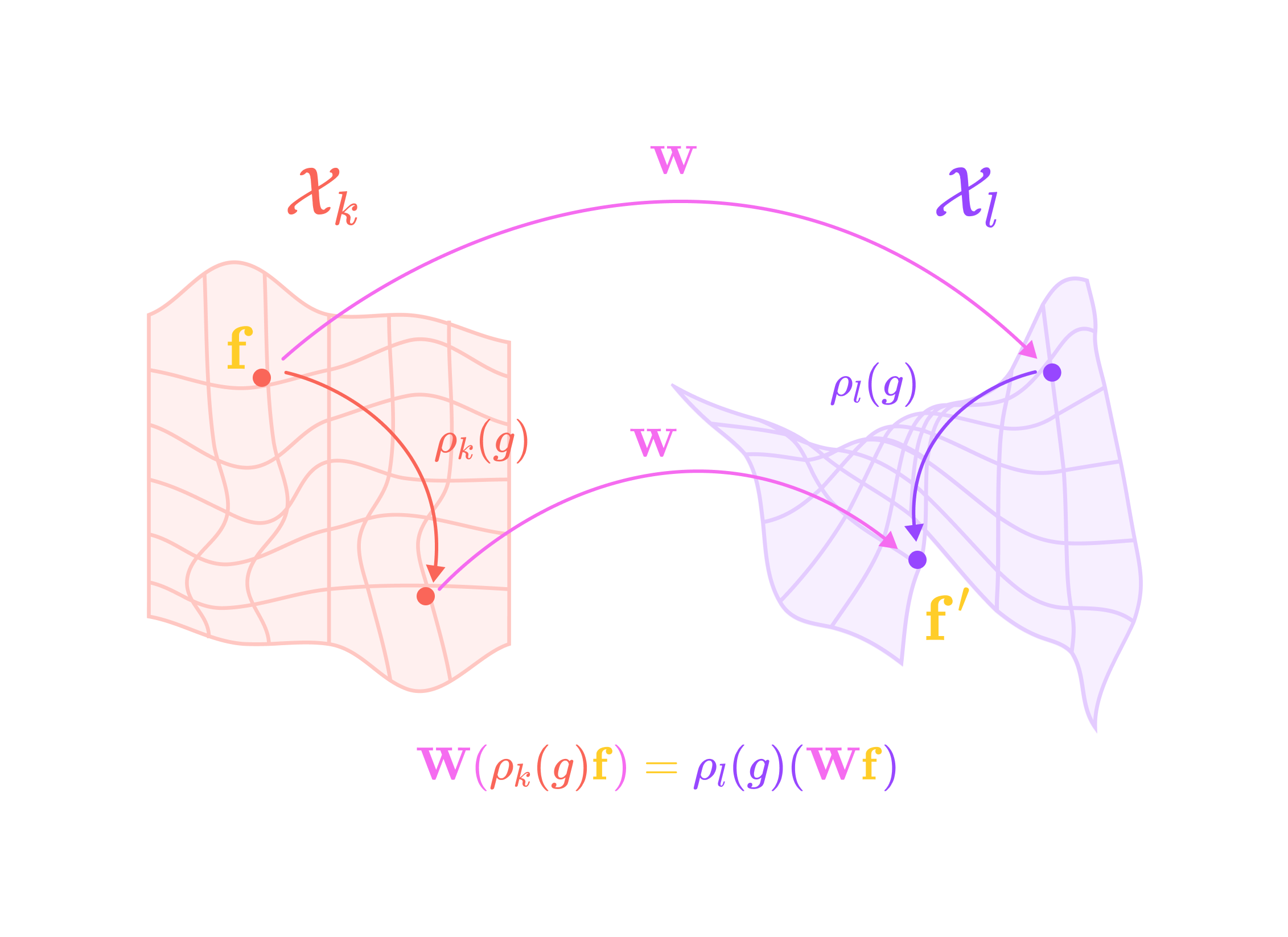
A function W that acts on a vector f is invariant under a group G if the output is the same before and after the action g in G is applied to the input, for all actions in the group.
A function is equivariant under group G if the output of the function also undergoes the same action g when the input is transformed by g.
ρ_k and ρ_l are group representations of G, where ρ_k acts in the same subspace Xk as the vector f and ρ_l acts in the same subspace Xl as the output of the function W.
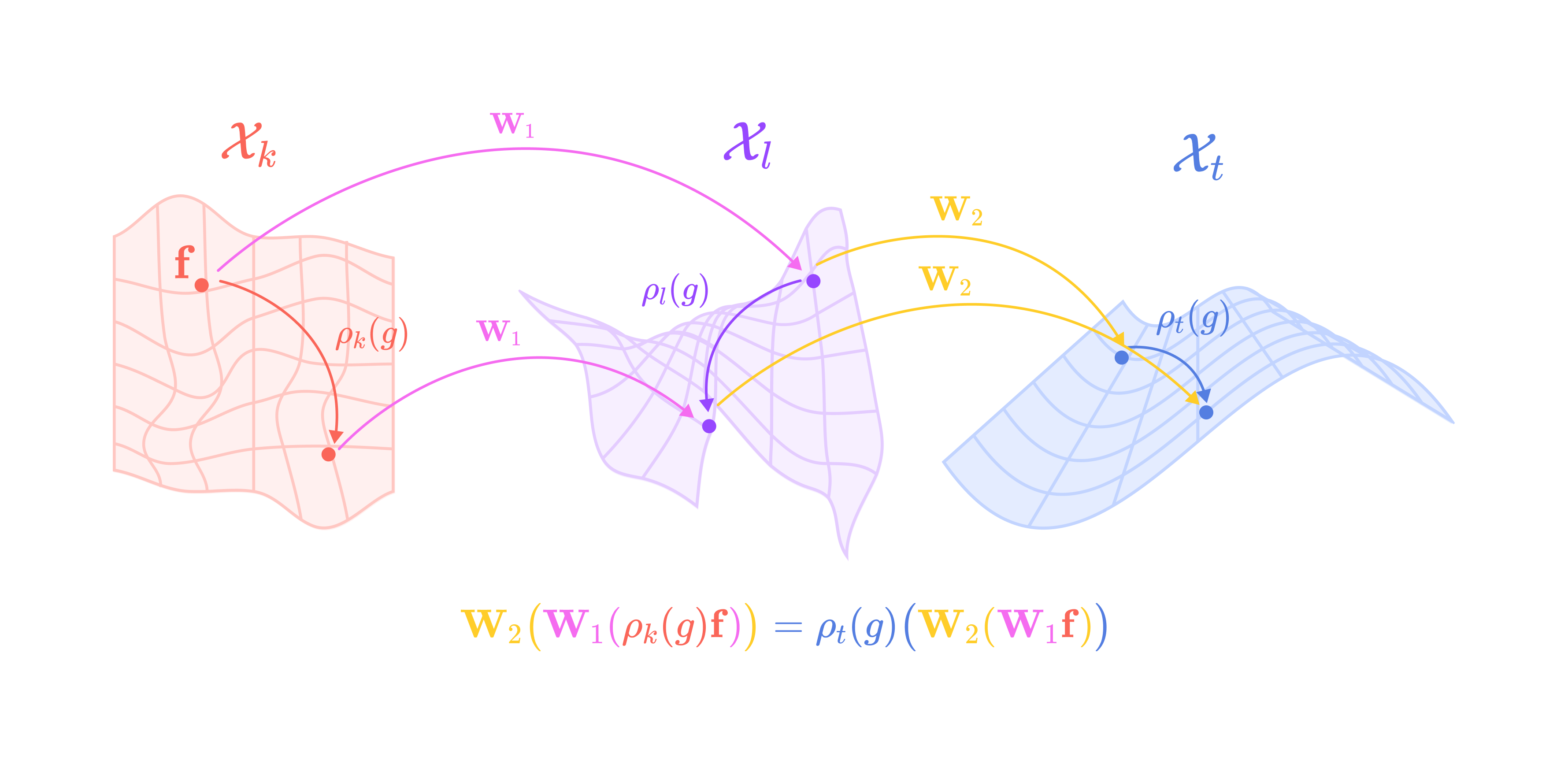
Applying two or more equivariant functions subsequently (or composing the functions) still satisfies the equivariance condition:
W2 is a second equivariant function applied after W1 that transforms the input from the subspace Xl to the subspace Xt.
This property allows us to compose as many equivariant functions as we want without worrying about breaking equivariance.
Functions in geometric GNNs should satisfy three types of equivariance in 3D: permutation equivariance, translation equivariance, and rotation equivariance. Permutation equivariance states that permuting the indices of nodes should permute the output or produce the same output (permutation invariance). In most GNNs, nodes are treated as sets of objects rather than an ordered list, so these models are inherently permutation invariant.
Since geometric graphs represent isolated systems defined by relative displacement vectors and not absolute spatial information, geometric GNNs are by default translation invariant, meaning shifting the position of all nodes in the graph by a displacement vector does not change the output. Unfortunately, satisfying rotational equivariance in 3D is a lot more challenging, making it the focus of advancements in equivariant models.
Spherical Tensors
The Special Euclidean Group in 3D, known as the SE(3) group, is the set of all rigid 3D transformations, including rotations and translations. We will be focusing on the subset of SE(3) called the Special Orthogonal Group in 3D, known as the SO(3) group, which is the set of all 3D rotations.
A representation of SO(3) is a set of invertible N x N square matrices that assign a specific matrix to every possible 3D rotation defined by the three Euler angles alpha α, beta β, and gamma γ. These angles define the rotation angles about the x, y, and z-axes, respectively.
These matrices or orthogonal and have a determinant of 1, meaning they preserve length and relative angles between vectors.
Since higher-dimensional tensors require more complex representations, we need a way of decomposing complex representations into smaller building blocks that can be used to rotate across tensors of increasing dimensions. These building blocks are called irreducible representations (irreps) of SO(3), which is a subset of rotation matrices that can be used to construct larger rotation matrices that operate on higher-dimensional tensors.
All group representations can be decomposed into the direct sum ⊕ (concatenation of matrices along the diagonal) of irreps. This block diagonal matrix can then be used to transform a higher-dimensional tensor after first applying an N x N change of basis matrix Q. Thus, we can write all representations of SO(3) in the following form:
In the equation above, Q is decomposes the input tensor into a direct sum of type-J spherical tensors aligned with each block in the block-diagonal Wigner-D matrix, and the transpose of Q converts the rotated spherical tensors back into their original basis.
There is a special subset of tensors called spherical tensors that transform directly under the irreps of SO(3) without the need for a change in basis.
Spherical tensors are considered irreducible types because all Cartesian tensors can be decomposed into their spherical tensor components, but spherical tensors cannot be decomposed further. Spherical tensors have degrees numbered by non-negative integers l that we call the tensor type. Type-l tensors are (2l + 1)-dimensional vectors that transform under a corresponding set of type-l irreducible representations of SO(3). We will describe both of these ideas more explicitly in the upcoming sections.
In quantum physics, spherical tensors are used to represent the orbital angular momentum of quantum particles like electrons. The degree of spherical tensors corresponds to the angular momentum quantum number (conventionally denoted with the letter l) that indicates the magnitude of angular momentum and the dimensions correspond to the (2l + 1) possible magnetic quantum numbers, which have integer values ranging from -l to l (denoted with the letter m) and is equal to the projected angular momentum on the z-axis relative to an external magnetic field.
Since angular momentum can be represented as a vector in 3D space, the value of m must be between -l (directly opposing the magnetic field) and l (perfectly aligned with the magnetic field), and since angular momentum is quantized, m must be an integer. In physics, |l,𝑚⟩ is used to denote a specific dimension m of a type-l spherical tensor which represents an eigenstate of a quantum particle, where the angular momentum is considered to be well-defined (more on this later).
Since the concepts of SO(3)-equivariance are deeply intertwined with quantum physics, specifically the coupling of angular momentum in quantum systems, I will continue to make connections to quantum mechanics throughout the article in these quotation blocks.
From Point Cloud to Geometric Graph
A point cloud is a finite set of 3D coordinates (or 3-dimensional vectors) where every point has a corresponding feature vector. Nodes can represent atoms in molecules, residues (C-alpha atoms) in proteins, or any unit in a system that carries information about itself in the form of feature tensors.
The feature vector f corresponding to each node in the point cloud contains data on its properties (e.g., atomic number, charge, hydrophobicity, etc.). The feature vector can be arranged into a tensor list, a multi-dimensional list of spherical tensors with three axes in the following order: a tensor axis, a channel axis, and a tensor-component axis.
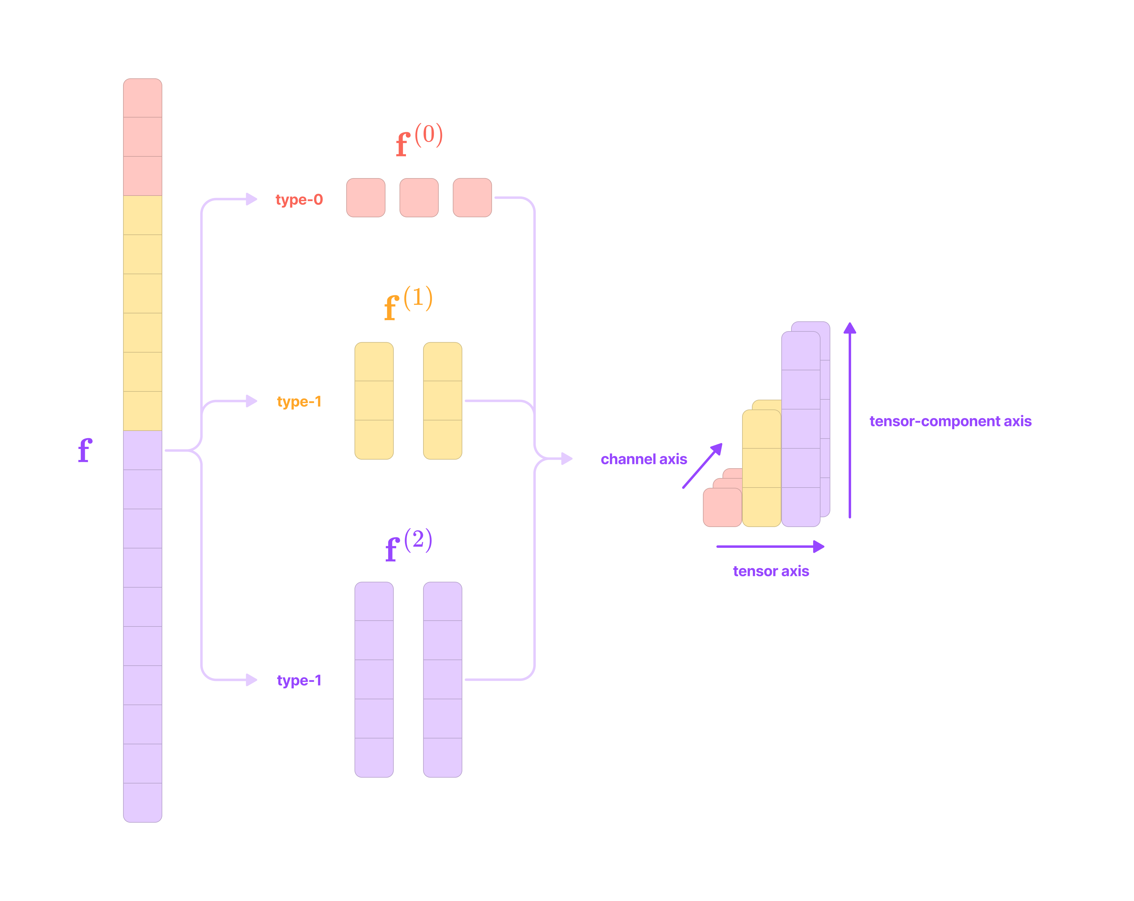
The channel axis represents the number of features of each type at the node. If a node contains three type-2 features, that feature has 3 channels.
The tensor axis represents the number of different types of spherical tensor features at the node. If a node has type-0, type-1, and type-2 features, it has a tensor axis dimension of 3.
The tensor-component axis represents the dimensions of each type of spherical tensor. For the type-k spherical tensors at the node, the tensor-component axis has dimension 2k + 1. Type-0 tensors are 1-dimensional scalars, type-1 tensors are 3-dimensional vectors, type-2 tensors are 5-dimensional vectors, and type-k tensors are (2k+1)-dimensional vectors.
From the point cloud, we want to generate a directional graph that contains directional edges between nodes that point in the direction of message-passing. An edge in the point cloud is defined by a displacement vector that points from node j (source node or neighborhood node) to node i (destination node or center node).
This can be decomposed into the radial distance (scalar distance between nodes) and the angular unit vector (vector with length 1 in the direction of the displacement vector). In the upcoming sections, we will see how both components are incorporated in constructing the equivariant kernel for message-passing.
Note that in most geometric graphs, edges are bidirectional, meaning there is an edge from node i to node j and an edge from node i to node j. The displacement vector of bidirectional edges has the same radial distance and angular unit vectors pointing in opposite directions.
Another way of representing a point cloud is as a continuous function f that takes in a 3-dimensional vector representing a point in 3D space (x) and outputs a feature vector (f) if x is in the point cloud (x = xj) or the zero vector if x is not in the point cloud.
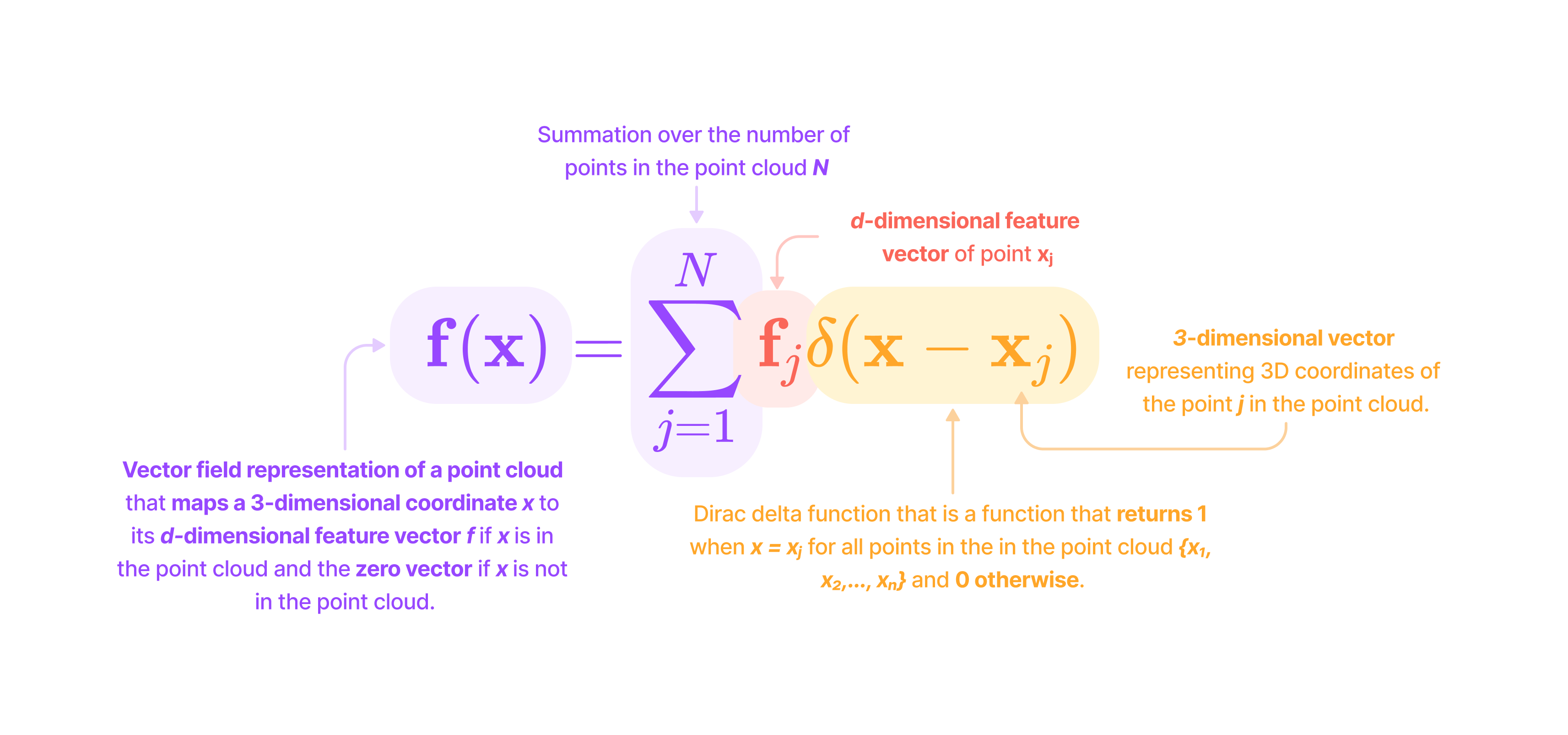
Since point clouds are defined by the relative spatial displacements between nodes in a global (non-fixed) reference frame, they often represent objects with rotational symmetries that must be handled equivariantly. This means that rotating the entire point cloud should generate rotated system-level outputs, and rotating individual nodes should generate rotated node-level updates.
Representing graphs as continuous functions facilitates continuous convolutions that are applied to every point in space, also known as point convolutions. However, for the sake of clarity, we will be considering graphs as a finite set of points on which the convolutions (which we will refer to as kernels) are applied. We do this by using summation notation, which will become clear in later sections.
Wigner-D Matrices
An irreducible representation (or irrep) of SO(3) defines how a type-l spherical tensor transforms under 3D rotation. The type-l irrep is a set of (2l + 1) x (2l + 1) matrices called Wigner-D matrices that rotate a type-l spherical tensor by an element g ∈ SO(3). For a specific 3D rotation g ∈ SO(3), the Wigner-D matrices for type-l tensors can be denoted as:
Type-0 tensors are scalars and remain unchanged under 3D rotation. The Wigner-D matrix for a type-0 vector is a 1 x 1 matrix with a single entry of 1.
\(\mathbf{D}_0(g)=[1]\)Type-1 tensors are 3-dimensional vectors and simply transform by the standard 3 x 3 rotation matrices under 3D rotation. All rotation matrices R, and thus Wigner-D matrices for type-1 tensors, can be constructed by multiplying the basic rotation matrices that rotate by an angle α about the x-axis (Rx), β about the y-axis (Ry), and γ about the z-axis (Rz).
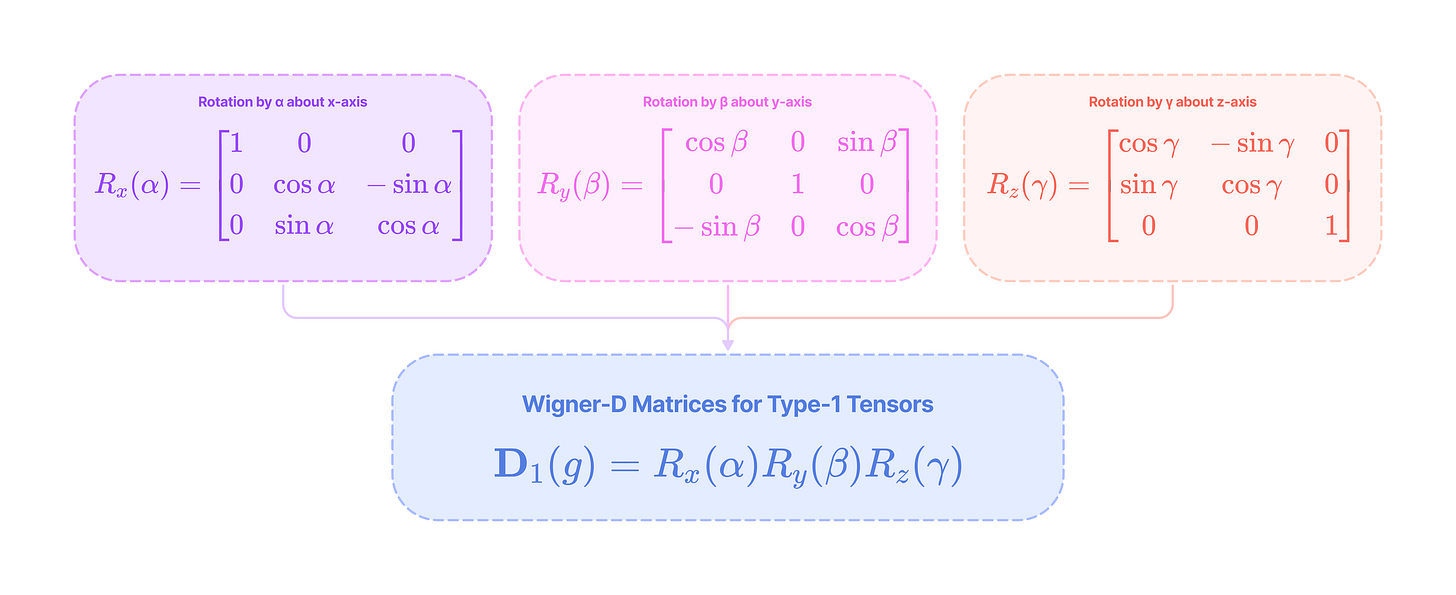
Type-1 Wigner-D matrices can be written as the product of the three standard rotation matrices around the x, y, and z-axis that transform 3-dimensional vectors. (Source: Alchemy Bio) Higher-order tensors (l > 2) transform by the corresponding (2l + 1) x (2l + 1) type-l Wigner-D matrix that we denote with a subscript l.

Now, we can define the equivariance condition using Wigner-D matrices. A function (or kernel), which we will denote as W, that transforms a type-k spherical tensor to a type-l spherical tensor is equivariant if it satisfies the following equivariance condition:
Since the feature vector is a stack of spherical tensors, it can be transformed via a matrix composed of concatenated Wigner-D matrices along the diagonal.
In the later section on tensor products, we will learn how to decompose any Cartesian tensor into its spherical tensor components, enabling them to transform directly and equivariantly under the Wigner-D matrices.
Spherical Harmonics
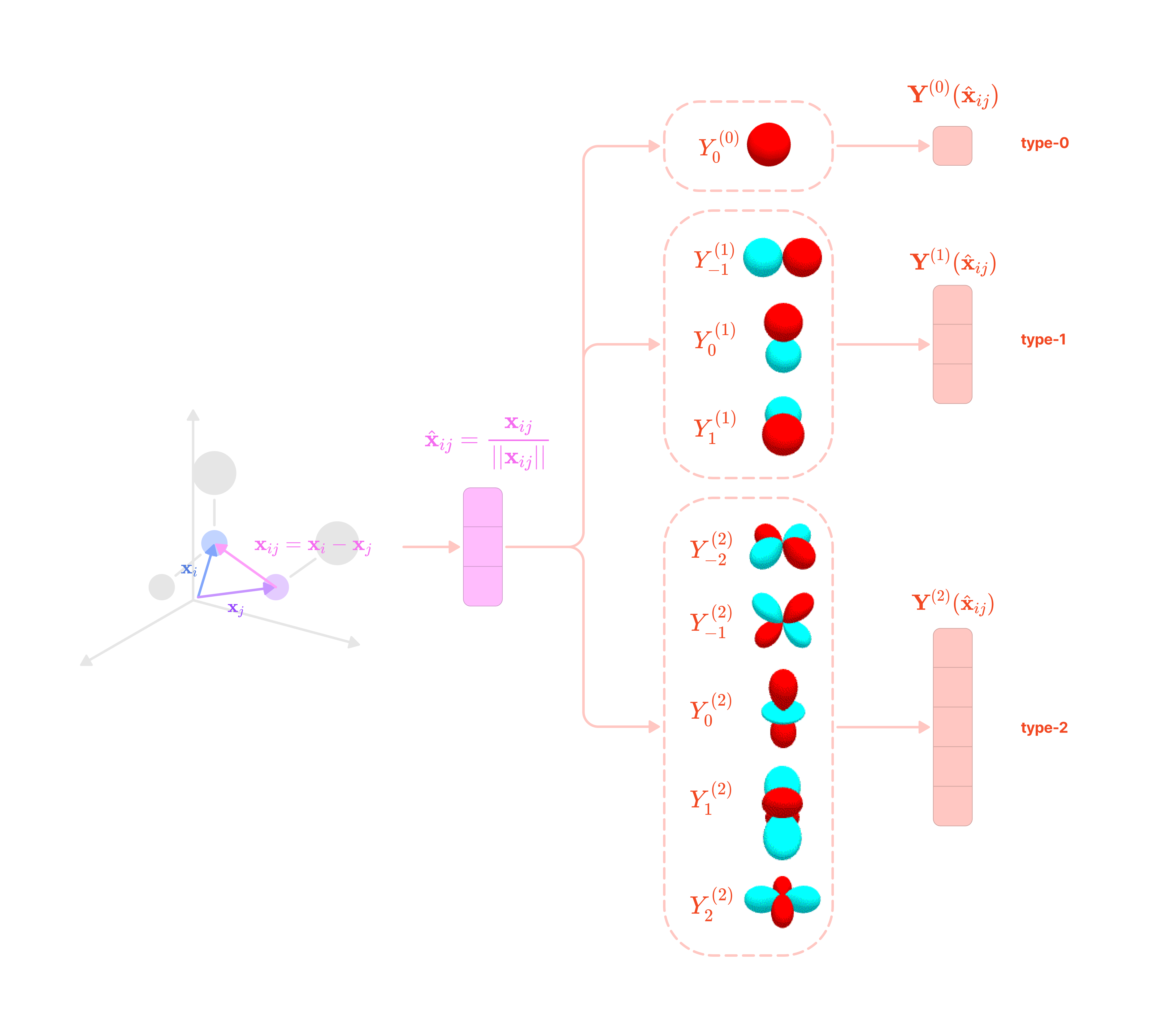
Spherical harmonics represent a complete and orthonormal basis for rotations in SO(3). They are functions that project 3-dimensional vectors into spherical tensors that transform equivariantly and directly under Wigner-D matrices, without requiring a change in basis. A spherical harmonic evaluated on a rotated 3-dimensional unit vector is equal to evaluating the spherical harmonic on the unrotated vector and transforming the output by an irrep of SO(3). Vectors of spherical harmonic functions are used to project the angular unit vector to spherical tensors, which are a fundamental building block of equivariant kernels.
The orthonormal basis functions with which all SO(3)-equivariant spherical tensors can be constructed are called spherical harmonics. We can also consider spherical harmonics as sets of functions that project 3-dimensional vectors onto orthogonal tensor subspaces that Wigner-D matrices operate in.
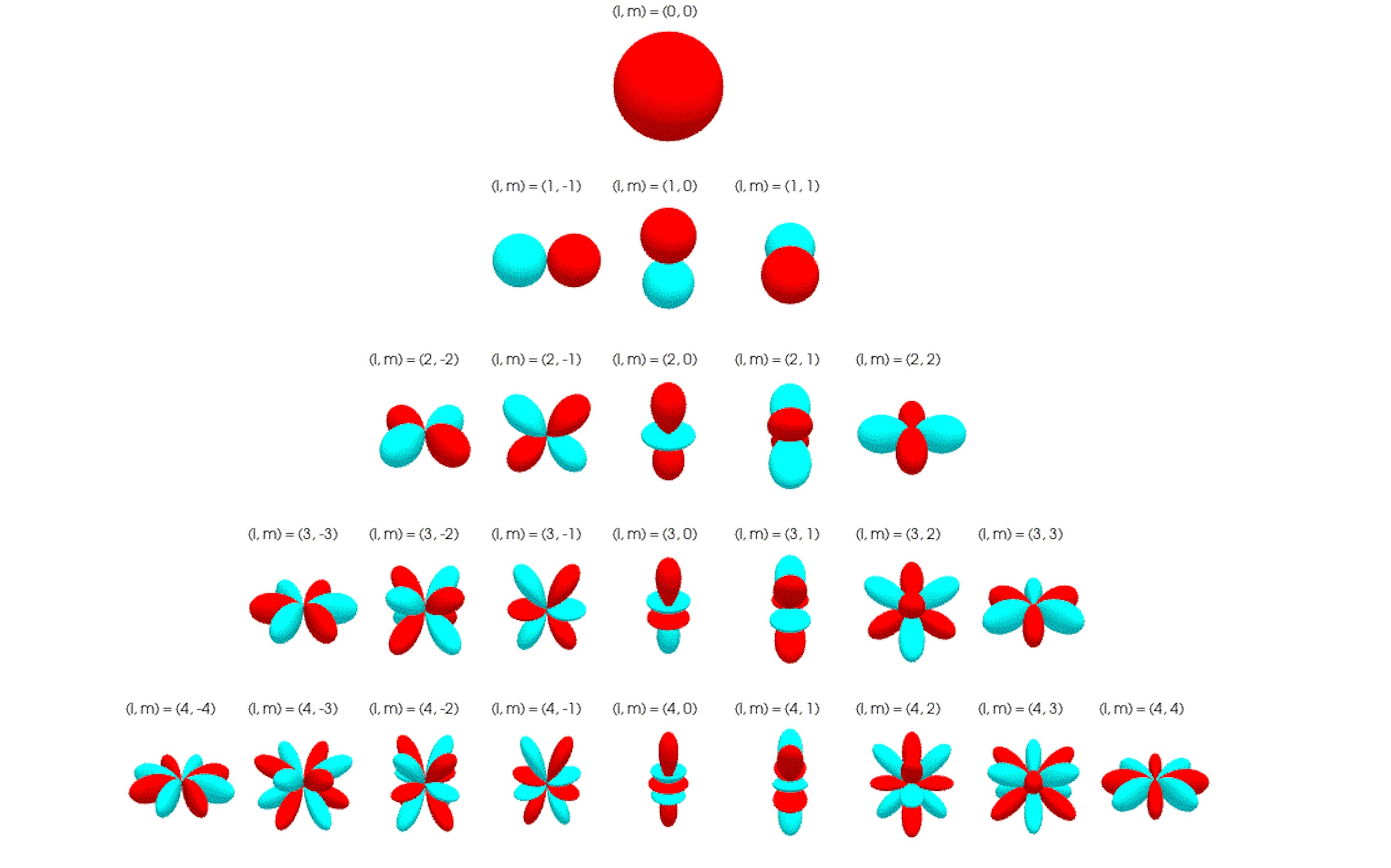
Each spherical harmonic function (indexed by its degree l and order m) takes a unit vector (length of 1) on the unit sphere (S²) and returns a real number.
For every type of spherical tensor l, there is a corresponding vector of 2l + 1 spherical harmonic functions indexed by m that transform points on the unit sphere into type-l spherical tensors that rotate directly under type-l Wigner-D matrices.
This spherical harmonic vector transforms a point on the unit sphere to a type-l spherical tensor:
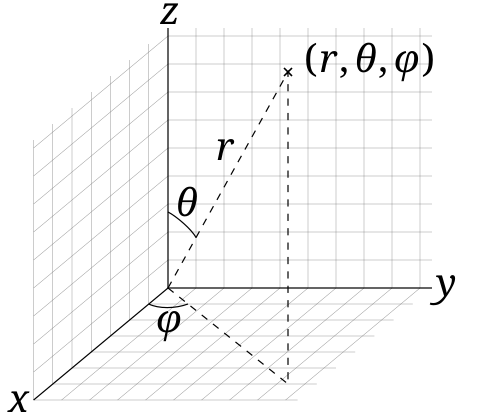
The explicit expressions defining the real spherical harmonics1 (or tesseral spherical harmonics) can be written in terms of the angle from the z-axis (polar angle θ) and the angle from the x-axis of the orthogonal projection onto the xy-plane (azimuthal angle φ):
The function dependent on cos(θ) is the associated Legendre polynomial (ALP) with degree l and order m given by the following equation:
In the equation above, Pl denotes the Legendre polynomial with maximum degree l. Visually, you can think of the Legendre polynomial where x=cos(θ) as a wave on the unit sphere. The zeros of the polynomial between [-1, 1] are nodes on the spherical harmonic where the harmonic changes sign. The set of Legendre polynomials is mutually orthogonal over the interval [-1, 1], meaning that the inner product of any two polynomials in the set is 0.
The Legendre polynomials are also complete, such that all square-integrable2 functions on the interval [-1, 1] can be approximated as a linear combination of the Legendre polynomials, where the coefficients are independent of one another.
When x=cos(θ), the (1-x²) term becomes sin²θ, and we can rewrite the ALP as:
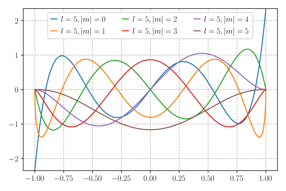
The associated Legendre polynomials (ALPs) are obtained by taking the mth derivative of the Legendre polynomials and scaling by a factor of (sinθ)ᵐ. Since the (sinθ)ᵐ factor is zero for θ = 0 (north pole) and θ = π (south pole) for all non-zero m, there is a node at the north and south poles. As the exponent m increases, the ALPs start to approach zero farther from the poles, and the peak between 0 and π becomes narrower, effectively decreasing the number of possible nodes between θ = 0 and π generated from the Legendre polynomial term. These properties are reflected in the graph below of all the ALPs of degree l=5 with non-negative orders of m.
The purpose of including the ALP in spherical harmonics as opposed to the unmodified Legendre polynomials is to allow dependence on the azimuthal angle (φ). Since the azimuthal angle is undefined at the poles, the (sinθ)ᵐ factor ensures that there is no contribution from the azimuthal term at the poles for all non-zero values of m.
When m = 0, the (sinθ)ᵐ factor is 1, and the polynomial is unbounded at the poles, and there is no azimuthal dependence in the spherical harmonic.
Including the sine or cosine function dependent on the azimuthal angle allows spherical harmonics to describe a larger range of functions on the sphere and orientations of the angular momentum vector in a magnetic field.
It is also worth noting that taking the lth derivative of a degree-l Legendre polynomial is a constant, and taking even higher order derivatives returns zero. This means that including the ALP term aligns with the condition that the magnitude of the angular momentum projected on the z-axis |m| must be less than the magnitude of the angular momentum vector |m| <= l.
Spherical harmonics inherit the properties of the Legendre polynomials and ALPs applied to the unit sphere, forming a complete and orthogonal basis for spherical tensors with the following properties:
The completeness of spherical harmonics means that all Cartesian tensors can be represented as a set of orthogonal projections on the spherical tensor subspaces that rotate directly under Wigner-D matrices via a change of basis.
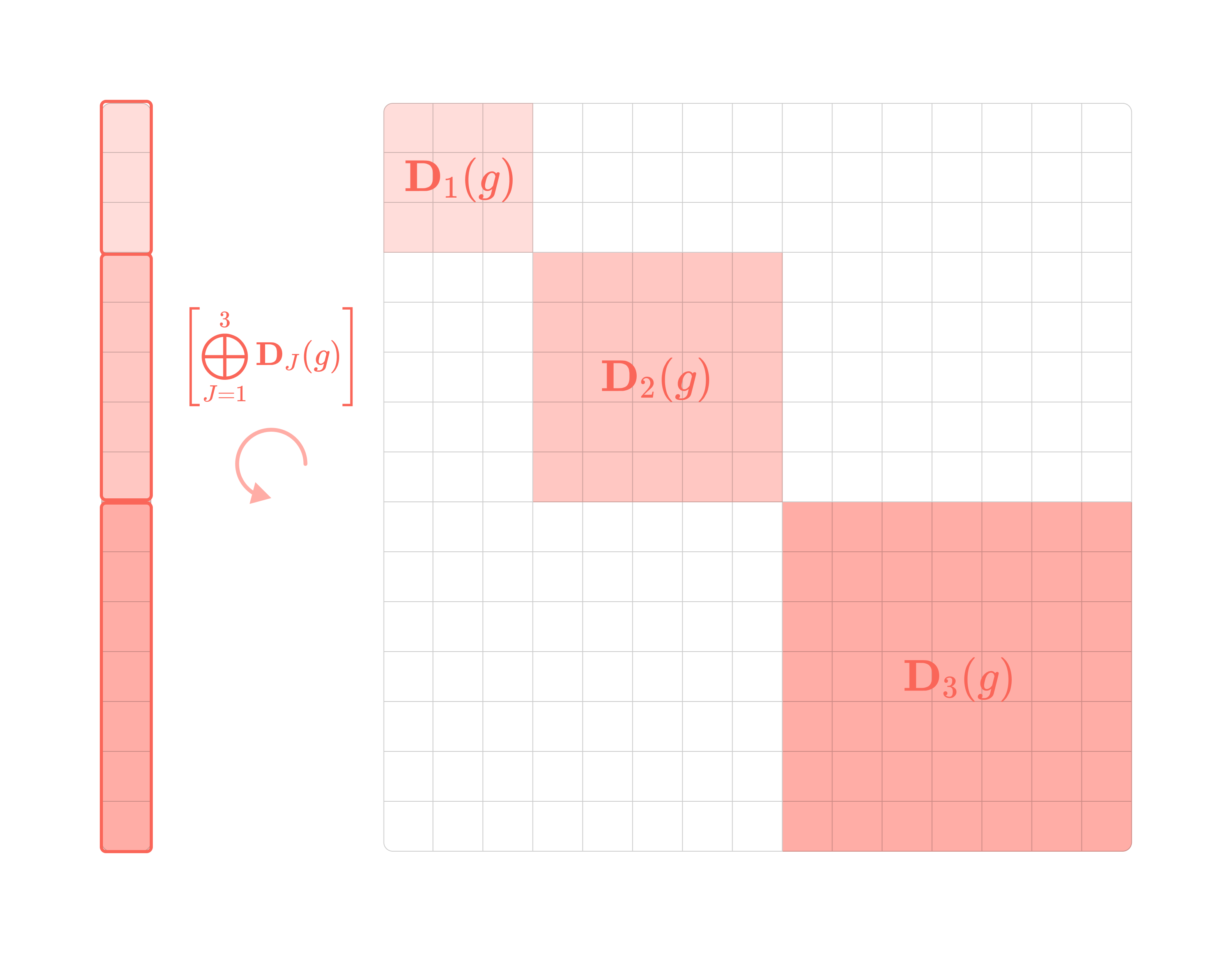
The orthogonality of spherical harmonics means that each type of spherical tensor transforms independently under rotation by the type-l Wigner-D matrix. This means that the direct sum (or vector concatenation) of spherical tensors rotates under a block-diagonal matrix with Wigner-D matrices along the diagonal and zeros everywhere else. The zero entries indicate that there are no cross dependencies between the tensors under rotation, a crucial property for our upcoming discussion on constructing equivariant layers.
\(\int_{S^2}Y^{(l)}_{m_l}(\theta,\phi)Y^{(k)}_{m_k}(\theta,\phi)d\Omega=\delta_{lk}\delta_{m_lm_k}\)The integral of the product of spherical harmonics over the unit sphere (inner product) is equal to the product of two Kronecker delta δ, which is equal to 1 if l = k or m_l = m_k, and zero otherwise. This means that the inner product of two real spherical harmonics is non-zero only when they share the same degree l and order m, and is zero for all distinct pairs of l and m.
To gain some physical intuition, let’s describe the role of spherical harmonics in quantum mechanics, where they are used to describe the angular component of electron wavefunctions.
Spherical harmonics are eigenfunctions of the orbital angular momentum operators L² and Lz that act on electron wavefunctions. When the squared total angular momentum operator (L²) is applied to a spherical harmonic, it returns the function scaled by the eigenvalue (scalar) ℏ²l(l+1) consisting of the total angular momentum number l, where ℏ is the Planck constant.
\(\hat{L}^2Y_m^{(l)}(\theta,\phi)=l(l+1)\hbar^2Y_m^{(l)}(\theta,\phi)\tag{$l=0,1,\dots$}\)In addition, when the z-component angular momentum operator (Lz) is applied to a spherical harmonic, it returns the function scaled by the eigenvalue mℏ containing the magnetic quantum number m.
\(\hat{L}_zY^{(l)}_m(\theta,\phi)=m\hbar Y^{(l)}_m(\theta,\phi)\tag{$m=-l,\dots,l$}\)These eigenvalues give the quantized values of orbital angular momentum, that is the angular momentum of an electron orbital cannot take any value but is limited to certain quantities defined by the integer values of l and m.
The orbitals with defined angular momentum |l,𝑚⟩ are called eigenstates, and they have wavefunctions that map every point in space to a probability amplitude. The square of the wavefunction describes the probability of an electron existing in a specific quantum state. Wavefunctions can describe the probability distribution of position, angular momentum, spin, or energy of an electron. The spherical harmonic corresponding to |l,𝑚⟩ is the angular component of the wavefunction of an isolated electron which describes how the probability densities vary with orientation around the origin.
This illustrates how spherical harmonics capture the foundational rotational symmetries of physical systems, which make them the perfect basis for constructing functions on the sphere that detect rotationally symmetric patterns in graph features. Watch this video to learn how to derive the first few spherical harmonics.
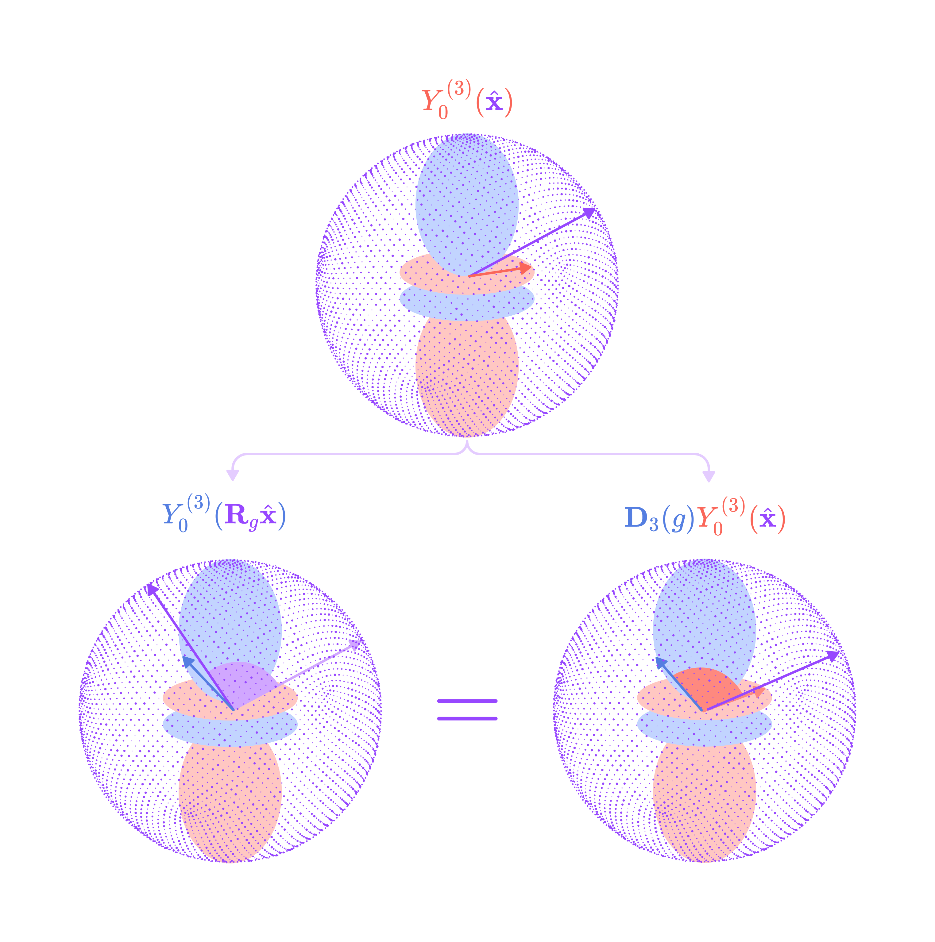
Critically, the spherical harmonics are equivariant functions, meaning that a rotation of the input 3-dimensional vector by the 3 x 3 rotation matrix R for g ∈ SO(3) is equivalent to rotating the spherical harmonic projection by the type-l Wigner-D matrix for g.
The type-J vectors of spherical harmonic functions with elements m = -J to J are used to project angular unit vectors of edges into higher-degree spherical tensors that can model different frequencies of rotationally symmetric features. These higher-degree spherical tensors form the basis set of SO(3)-equivariant kernels that can combine to capture complex rotationally symmetric chemical properties with high precision, which we will discuss in depth later in the article.
Like how the Fourier series decomposes periodic signals into sine and cosine components with specific periodic frequencies, spherical harmonics decompose rotationally symmetric, or SO(3)-equivariant, features on the unit sphere into components that change with specific angular frequencies. This decomposition is crucial to model how SO(3)-equivariant features vary across positions and orientations on the unit sphere.
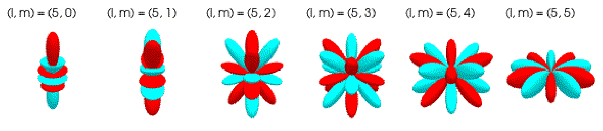
The degree or type of a spherical harmonic determines its frequency or how rapidly it oscillates on the sphere. Lower-degree harmonics can model features with broader, smoother variations under rotations, while higher-degree harmonics capture features with sharper, finer variations under rotation.
Just as low-frequency sinusoids fail to accurately approximate high-frequency functions in Fourier analysis, low-degree spherical harmonics are not sensitive enough to handle chemical properties that vary dramatically with subtle changes in atomic orientation and position.
In the later section on computing the basis kernels, we will deconstruct how to precompute the spherical harmonic functions using recursive relations.
Now that we have defined the basis for spherical tensors, let’s discuss how to combine and convert between tensors of different types using the tensor product.
Tensor Product
The tensor product is a bilinear and equivariant operation that combines two spherical tensors to produce a higher-dimensional tensor. Since the output higher-dimensional tensors are generally not spherical tensors themselves, we must decompose them into their spherical tensor components using change-of-basis matrices formed with Clebsch-Gordan coefficients.
Suppose we want to exchange information between type-k and type-l features. Since they are different types, they are transformed differently under 3D rotation. How do we exchange information between these features without breaking equivariance?
This is where the tensor product comes in, which is denoted by ⊗.
The tensor product converts the type-k and type-l spherical tensors into a (2l+1) x (2k+1) matrix by calculating the product of every pair of dimensions indexed by m_k and m_l.
We can flatten this matrix into a (2l+1)(2k+1)-dimensional tensor. However, this higher-dimensional tensor is not spherical, and we must define the representation D(g) under which it rotates equivariantly. Since the tensor product is equivariant, it satisfies the equivariance condition, which states that rotating the tensor product by g is equivalent to rotating the individual spherical tensors by their respective Wigner-D matrices and then taking the tensor product. This translates into the following equation:
Using the tensor product identity below:
We can manipulate the above equation to isolate the Wigner-D matrices:
This means that the tensor product of a type-k and a type-l tensor rotates under the representation of SO(3) derived from the Kronecker product (⊗) of the type-k and type-l Wigner-D matrices:
The Kronecker product operation is analogous to the tensor product for matrices that produces a ‘matrix of matrices’ where each block of the outer matrix is an inner matrix derived from scaling the second matrix in the product by the corresponding element of the first matrix.
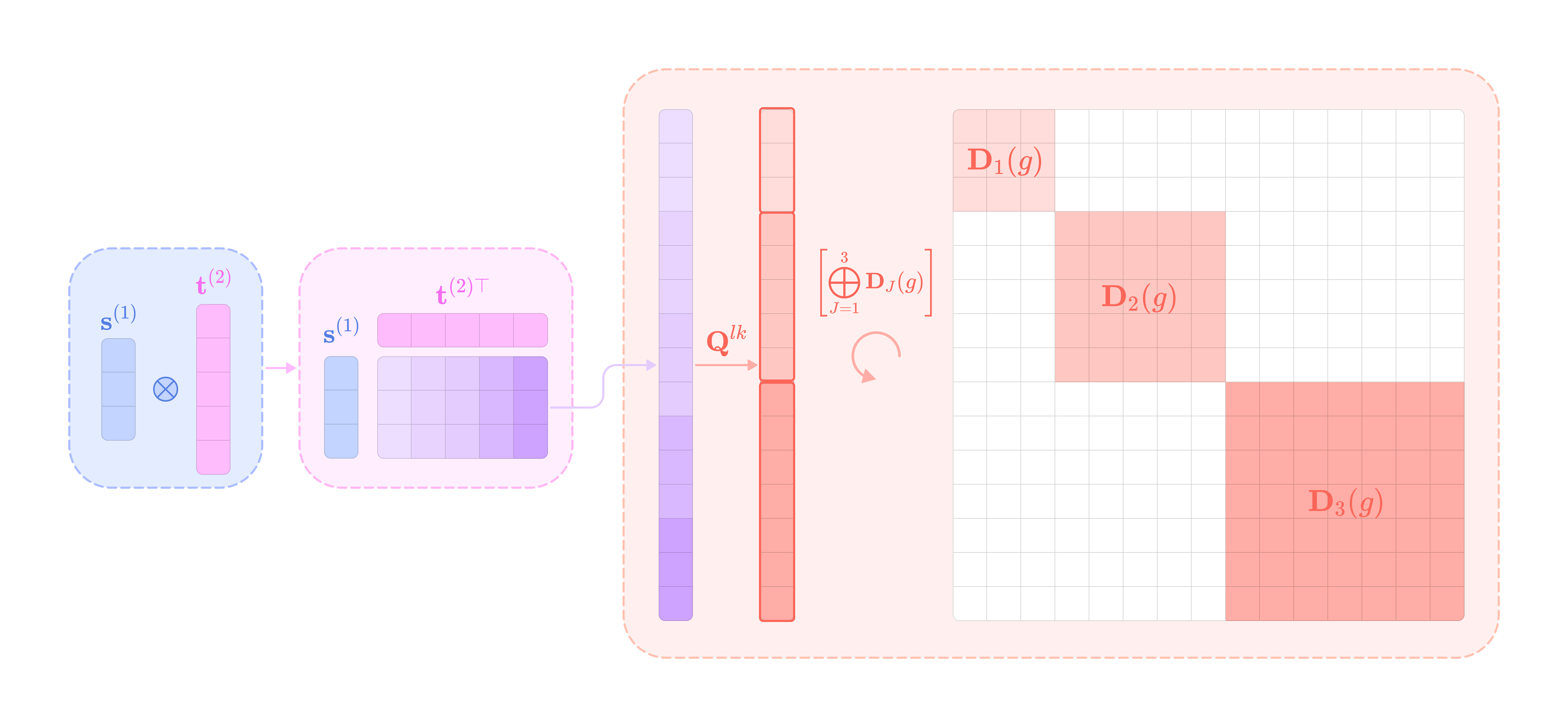
The Kronecker product of two SO(3) representations is another representation; but since every group representation can be written as the direct sum of irreps (where each block along the diagonal is an irrep and the remaining entries are zero) coupled with an orthogonal change-of-basis matrix and its transpose, we can decompose the Kronecker product of the type-k and type-l Wigner-D matrices into the direct sum of Wigner-D matrices coupled with the change of basis matrix composed of a special set of coefficients called the Clebsch-Gordan coefficients (which we will dive into in the next section).
where Q is a (2l+1)(2k+1) x (2l+1)(2k+1) orthogonal change-of-basis matrix where each element is a Clebsch-Gordan coefficient.
From this equation, we see that the Clebsch-Gordan change of basis matrix can be used to transform the (2l+1)*(2k+1)-dimensional tensor product into the direct sum of exactly one spherical tensor of each type ranging from |k-l| to k+l stacked into a single vector that rotates under the direct sum of Wigner-D matrices ranging from |k-l| to k+l. We can think of the change-of-basis operation as projecting the tensor from the combined space into several orthogonal subspaces that rotate under defined representations of SO(3).
Let’s solidify this abstract idea with a familiar example. Consider the tensor product of two type-1 tensors (3-dimensional vectors) a and b, which gives a 3 x 3 matrix (or 9-dimensional tensor):
We can extract some familiar values from this matrix:
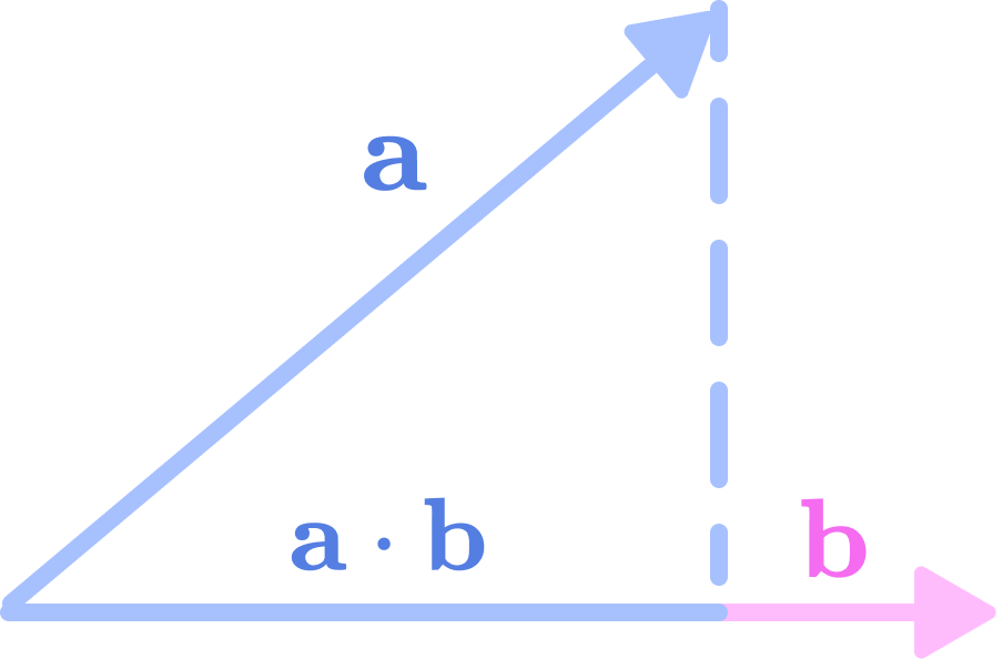
We can see that the trace of the matrix (sum of values along the diagonal) is equal to the dot product of a and b.
\(\mathbf{a}\cdot \mathbf{b}=a_xb_x+a_yb_y+a_zb_z\)
The dot product of two 3-dimensional vectors a and b is the length of the projection of a onto the line spanned by b. The dot product is invariant to rotation. (Source: Alchemy Bio) The dot product can be interpreted as the length of the projection of the vector a on the line created by vector b. If we rotate both a and b, the length of the projection shouldn’t change because the lengths of the individual vectors and the angle between them remain constant under rotation. So we can think of the trace as the type-0 spherical tensor component of the 9-dimensional Cartesian tensor that transforms invariantly under rotation.
We can also extract the cross-product from this 3 x 3 matrix from the antisymmetric elements:
\(\mathbf{a}\times \mathbf{b}=\begin{bmatrix}a_yb_z-a_zb_y\\a_zb_x-a_xb_z\\a_xb_y-a_yb_x\end{bmatrix}\)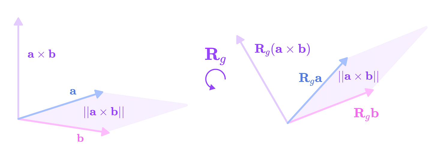
The cross product between two 3-dimensional vectors a and b is the vector perpendicular to both a and b (direction obtained from the right-hand rule) with a magnitude equal to the area of the parallelogram formed by the two vectors. The cross product is equivariant under rotation by the type-1 Wigner-D matrices. (Source: Alchemy Bio) The cross-product can be interpreted as the vector perpendicular to both vectors a and b with length equivalent to the area of the parallelogram formed by the two vectors. If we rotate a and b by the rotation matrix R, the cross-product should rotate by the same matrix R but the length would remain constant since rotations preserve lengths and angles. Thus, we can think of the cross product as the type-1 spherical tensor component of the 9-dimensional Cartesian tensor that transforms under the type-1 Wigner-D matrices (standard 3 x 3 rotation matrices).
Unfortunately, the type-2 spherical tensor component of the 3 x 3 matrix does not have a concrete physical interpretation. However, we can think of it as the traceless, symmetric part of the matrix that rotates under the type-2 Wigner-D matrices.
\(\begin{bmatrix}c(a_xb_z+a_zb_x)\\c(a_xb_y+a_yb_x)\\2a_yb_y-a_xb_x-a_zb_z\\c(a_yb_z+a_zb_y)\\c(a_zb_z+a_xb_x)\end{bmatrix}\)
The decomposed 9-dimensional Cartesian tensor is the direct sum of the type-0 (trace), type-1 (asymmetric), and type-2 (traceless, symmetric) spherical tensor components.
If we stack all three representations into a (1+3+5)-dimensional tensor, the resulting vector concatenation rotates under the direct sum of the type-0, type-1, and type-2 Wigner-D matrices:
The tensor product in quantum mechanics is used to describe the overlap (or coupling) of two electron orbitals with well-defined angular momentum states |l, 𝑚_l⟩ and |k, 𝑚_k⟩. These are considered angular momentum eigenstates, because the values the total angular momentum (l and k) and magnetic quantum number (m_l and m_k) are eigenvalues of the angular momentum operators with their eigenfunction being the corresponding spherical harmonic function. Since angular momenta are vector quantities, we can consider the uncoupled angular momentum vectors of each eigenstate as a 3-dimensional vector and the coupled angular momentum as the vector addition of the eigenstate vectors.
When the angular momentum vectors of both uncoupled eigenstates are perfectly aligned, their coupled state has a maximum momentum of k + l and when they are perfectly disaligned, their coupled state has a minimum magnitude of |k - l|. The two eigenstates can overlap in any relative orientation, so the magnitude of the angular momentum vector of the coupled state can theoretically be anywhere between these two boundaries.
However, we discussed earlier that angular momentum is quantized, and can only have discrete values corresponding to non-negative integer values of l and integer values of m from -l to l. This means that we can think of the coupled state as a probability distribution of coupled eigenstates with well-defined angular momenta corresponding to integer values of l between |k - l| to k + l. The m value of the coupled eigenstates must be equal to the sum of the uncoupled eigenstates (m = m_l + m_k) since the projection of angular momentum on the z-axis is a scalar value without directionality. The probabilities of finding each coupled eigenstate in the total coupled state are represented by the Clebsch-Gordan coefficients, which can be used to decompose tensor products (total coupled state) into their spherical tensor components (coupled eigenstates).
Clebsch-Gordan Decomposition
Now, we will define the Clebsch-Gordan coefficients (CG coefficients) that form the change-of-basis matrices transforming tensors from the combined tensor product space into their spherical tensor components.
First, let’s develop some intuition about the purpose of the CG coefficients in the context of angular momentum coupling.
As mentioned earlier, the coupled angular momentum state is a probability distribution of coupled eigenstates with well-defined angular momenta. Each Clebsch-Gordan coefficient indicates the amplitude of the wavefunction corresponding to an eigenstate |J, 𝑚⟩ in the wavefunction of the coupled state |l, 𝑚_l⟩|k, 𝑚_k⟩. The square of the absolute value of the CG coefficients is the probability of finding the eigenstate |J, 𝑚⟩ in the coupled state |l, 𝑚_l⟩|k, 𝑚_k⟩, which means the probabilities across all coupled eigenstates must sum to 1:
\(\sum_{J=|k-l|}^{|k+l|}|C^{(J, m)}_{(l, m_l)(k, m_k)}|^2=1\)Furthermore, we can obtain the wavefunction of the coupled eigenstate |J, 𝑚⟩ for a defined value of J as a linear combination of coupled states |l, 𝑚_l⟩|k, 𝑚_k⟩ for different values of m_l and m_k scaled by the CG coefficients.
\(|J, m⟩=\sum_{m_l=-l}^l\sum_{m_k=-k}^kC^{(J, m)}_{(l, m_l)(k, m_k)}|l, m_l⟩|k, m_k⟩\)
There are (2l + 1)(2k + 1)(2J + 1) CG coefficients needed for the decomposition from the tensor product to one type-J spherical tensor component, which can be represented as a (2l + 1)(2k + 1) x (2J + 1) matrix. This is only a slice of the (2l + 1)(2k + 1) x (2l + 1)(2k + 1) matrix needed for the decomposition of the tensor product for all values of J.
When decomposing the tensor product of a type-k and type-l tensor, each CG coefficient scales the product of the m_l dimension of the type-l tensor and the m_k dimension of the type-k tensor to give the mth dimension of the type-J spherical tensor component.
We can consider each CG coefficient C as a scaling factor that projects the (m_k, m_l) element of the tensor in the combined k ⊗ l tensor space to the orthogonal mth element of the orthogonal type-J spherical tensor subspace.
In a later section on computing the basis kernels, we will be breaking down how to calculate the Clebsch-Gordan change-of-basis matrices using the Sylvester equation.
Parameterizing the Tensor Product
A core mechanism of spherical equivariant geometric GNNs is combining tensors of various types with learnable weights and training them to learn rotationally symmetric relationships between nodes. To do this, we must introduce learnable parameters into the tensor product without breaking equivariance.
As we defined earlier, the tensor product of a type-k and type-l spherical tensor can be decomposed into k + l - |k - l| + 1 = 2min(l, k)+1 spherical tensors of types ranging from J = |k - l| to k + l. Since the output of the tensor product is no longer a spherical tensor, directly applying learnable weights to the tensor product will break equivariance since the elements do not transform predictably under rotation.
Instead, we can apply learnable scalar weights separately to each component of the decomposed spherical tensor components, since they are orthogonal and rotate independently under the irreps of SO(3).
The equivariance condition holds since the weight w is a type-0 scalar that is invariant to rotations.
We can define the parameterized tensor product of a type-k spherical tensor s and a type-l spherical tensor t as the direct sum of the type-J spherical tensor components each scaled by a weight indexed by the type of first input (k), the type of the second input (l), and the type of the component it is applied to (J) from the tensor product decomposition.
where the subscript J denotes the type-J component of the tensor product decomposition.
When taking the tensor product between two lists of spherical tensors of multiple channels of multiple feature types, we can think of the combination of a single tensor type from the first tensor list, a single type from the second tensor list, and the type of the decomposed tensor product component (k, l, J) as a path in the tensor product and assign a learnable parameter to each path. In the case above where we took the tensor product between a single type-k and type-l spherical tensor, the number of learnable weights equals the 2min(l, k) +1 possible values of J.

First, we will generalize to multi-type input tensors with a single channel of each type before extending to multiple channels in the section on Tensor Field Networks. The tensor product of the tensor list s of types ranging from k = 0 to K with the tensor list t of types ranging from l = 0 to L can be written as follows:
For every combination of input types (k, l) where k = 0 to K and l = 0 to L where J is in the range |k-l| to |k+l|, we extract the type-J component of the decomposed tensor product between the type-l channel and the type-k channel of the tensor list. Since each extracted type-J tensor corresponds to a single path (k, l, J), we scale the output with a unique learnable weight w.
Then, we take the element-wise sum of the weighted type-J tensors from every path (k, l, J) that share the same value for J, since they are all (2J+1)-dimensional and transform with the same irreps under rotation.
By repeating steps 1 and 2, we get a single tensor for every possible degree J from 0 to K+L, each of which is the weighted sum of all the decomposed type-J components generated from the tensor products between different combinations of degrees l and k from the input tensor lists.
These vectors can be concatenated into a single vector containing subvectors of types J = 0 to K+L.
Now, we can explicitly define each entry of the type-J spherical tensor component (m = -J to J) of the tensor product decomposition using the Clebsch-Gordan coefficients:
Let’s break down how to calculate the parameterized tensor product with an example that applies to equivariant kernels: the tensor product between the list of feature tensors and the list of spherical harmonics projections of the angular unit vector.
Suppose we have a feature list f that contains a type-0 and type-1 tensor. We also have the angular unit vector x̂ between nodes i and j projected into type-0 and type-1 tensors using the type-0 and type-1 spherical harmonics. We can denote each tensor list as a vector of stacked spherical tensors:
First, we can determine every path (l, k, J) that results in a type-J spherical tensor component for all possible values of J ranging from |0-0|=0 to 1+1=2.
Then, we compute the tensor products between every pair of tensors in the input lists, decompose them into their spherical tensor components, scale each path by a weight, and take the sum over all the outputs with the same degree.
The type-0 (J = 0) sum of the paths (0, 0, 0) and (1, 1, 0) is a scalar:
The type-1 (J = 1) sum of the paths (0, 1, 1), (1, 0, 1), and (1, 1, 1) is a 3-dimensional vector:
The type-2 (J = 2) output of the path (1, 1, 2) is a 5-dimensional vector:
Finally, we can concatenate each weighted sum into a single 9-dimensional vector to get the output of the tensor product between the feature tensor list and the list of spherical harmonics projections of the angular unit vector.
Review
Since we’ve covered quite a lot of concepts, let’s synthesize these concepts in the context of SO(3)-equivariance:
The group of rotations in three dimensions is called the SO(3) group and the group representations are N x N orthogonal matrices that can be decomposed into irreducible representations (irreps) called Wigner-D matrices.
Wigner-D matrices can act on any tensors after applying a change-of-basis matrix; however, they act directly on special types of tensors called spherical tensors that are generated by spherical harmonics. Spherical harmonics form a complete, orthonormal basis of functions on the unit sphere that can project vectors on the unit sphere to spherical tensors that can be transformed directly and equivariantly with Wigner-D matrices.
These special spherical tensors are divided into types (or degrees) that are denoted by a non-negative integer (l = 0, 1, …) and are 2l+1-dimensional. The Wigner-D matrices that act directly on type-l tensors have dimensions (2l+1) x (2l+1) and there is a set of 2l +1 spherical harmonic functions that project vectors into type-l tensors. Higher-degree spherical tensors change more rapidly under rotation and are represented by higher-frequency spherical harmonic functions on the unit sphere.
The tensor product is a tensor operator that transforms two lower-degree tensors into a higher-degree tensor. The tensor product of two spherical tensors is no longer a spherical tensor but can be separated into exactly one spherical tensor of each type, ranging from |k - l| to k + l by multiplication with a change of basis matrix containing Clebsch-Gordan coefficients.
The tensor product allows us to pass messages from a type-k feature from a neighborhood node to a type-l feature at the center node without breaking equivariance. This is done by extracting the type-l spherical tensor component of the tensor product between the type-k feature with a spherical tensor generated from spherical harmonics.
Weights or learnable parameters can only be applied after decomposing the tensor product into its spherical tensor components, which means a maximum of one parameter can be applied for every set of values (l, k, J) corresponding to the two input types and the tensor product component type, respectively.
Now, we will be putting these ideas into practice to generate an equivariant kernel that transforms between degrees of spherical tensors and generates messages between nodes.
Before getting started, the code implementation of SE(3)-Transformers uses a novel data structure called fibers to keep track of node and edge features. The structure of a fiber is a list of tuples that are used to define the degrees and number of channels that are inputted and outputted from equivariant layers in the form [(multiplicity or number of channels, type or degree)]. The code implementation will often extract a (multiplicity, degree) pair from a fiber structure in the following way:
You can find the full implementation of the data structure here.
Constructing an Equivariant Kernel
To facilitate message-passing between spherical tensors of different types, we want to construct a kernel that can take a single type-k input feature and directly transform it into a type-l feature.
In a non-equivariant setting, this is simple. All we need is to multiply by a (2l + 1) x (2k + 1) kernel of learnable weights to transform the (2k + 1)-dimensional type-k tensor to a (2l + 1)-dimensional type-l tensor. However, multiplying a randomly initialized kernel would break equivariance, so we must carefully define how to construct a kernel W of the same dimensions that linearly transforms type-k to type-l tensors while preserving SO(3)-equivariance.
This kernel should also be dependent on the displacement vector from node j to i which encodes the distance and relative angular relationship between the two nodes.
With these ideas in mind, let’s define the kernel W as a function that takes the displacement vector as input and outputs a (2l + 1) x (2k + 1) linear transformation matrix.
Deriving the Equivariant Kernel Constraint
To construct an equivariant kernel, we must first define how it must operate under rotations. I will be deriving the kernel constraint from scratch since it is the fundamental building block of equivariant GNNs. This section took a while for me to write as it forced me to wrestle with various notation-heavy derivations from publications, but I have broken it down to help you develop an intuitive understanding of the underlying concepts.
We know that W transforms a type-k input feature from node j to type-l features for message passing to node i:
This must satisfy the equivariance constraint on SO(3):
We can think of the kernel applied to a specified type-k feature as a tensor field. A field is a mathematical object that assigns a mathematical object to every point in space. In this case, for every point in 3-dimensional space (defined by the vector x), there is an assigned type-l tensor:
Rotating a tensor field is not as simple as rotating the tensors themselves since both the orientation and position of the tensors must rotate.
We can visualize this idea with an example: consider rotating the vector field f(x), which assigns a 3-dimensional vector to every point in 3D space by 90 degrees counterclockwise.
To rotate the vector field, we must perform two operations:
First, we shift the vector assigned to the point R⁻¹x to a new, rotated point 90 degrees counterclockwise from the original point x without changing its orientation. This is done by applying the inverse rotation matrix to the point x so that the vector field f(x) outputs the same vector as it would at the unrotated point.
Then, we rotate the vector at point x itself using the 3 x 3 rotation matrix R.
The rotated tensor field can be written with the following expression, where g denotes the 90-degree counter-clockwise rotation:
Let’s apply the same idea to rotate the tensor field expression by g.
First, we shift the tensor assigned to the unrotated point R⁻¹x to a new point rotated by g without changing its orientation by applying the inverse 3 x 3 rotation matrix to the point x. This sets the tensor assigned to the rotated point to be the same as the unrotated point. Then, we rotate the output type-l feature of the expression by the type-l Wigner-D matrix for g.
This gives us the definition of rotating the type-l output of the kernel by g in terms of the type-k input and the displacement vector:
Intuitively, when we rotate the point cloud, the kernel also changes since it is dependent on the displacement vector. However, we can only apply the equivariant condition on a ‘fixed’ function. This means that when applied in the same way to both an unrotated and rotated point cloud, the function can recognize rotated input features and operate on them equivariantly, such that the output is rotated accordingly. So we have to rotate the displacement vector back to its original frame to ensure that the kernel is defined the same way when operating on the rotated feature.
Now that we have defined how to rotate the entire tensor field expression by g, we can use it to rewrite the equivariance constraint defined earlier using our new definition for the rotated type-l output feature.
We can substitute x with the vector rotated by g:
and multiply the inverse of the type-k Wigner-D matrix on both sides to get:
The last line of the derivation above is called the kernel constraint because a kernel is SO(3)-equivariant if and only if it is a solution to the constraint, which is rewritten below for clarity:
We can convert the constraint into an equivalent matrix-vector form by vectorizing both sides and using the tensor product identity defined earlier with the property that Wigner-D matrices are orthogonal (its inverse is equal to its transpose).
As discussed previously, the Kronecker product of the type-k and type-l Wigner-D matrices (in this order) is a reproducible representation of SO(3) that acts on (2l+1)(2k+1)-dimensional tensors in a way that is equivalent to (1) applying a change-of-basis matrix Q that converts the tensor into the direct sum of spherical tensors of degree ranging from |k - l| to |k + l|, (2) applying the block diagonal matrix of the Wigner-D irreps corresponding to every degree ranging from |k - l| to |k + l|, and (3) changing the tensor back to its original basis. Q is an orthogonal (2l+1)(2k+1) x (2l+1)(2k+1) matrix that is composed of Clebsch-Gordan coefficients.
By multiplying both sides by Q and denoting the Clebsch-Gordan decomposition of the vectorized kernel with η, we can rewrite the equation as:
where:
Since η can be directly transformed by the block diagonal matrix of type |k - l| to |k + l| Wigner-D irreps without a change-of-basis, we know it must be the direct sum of spherical tensors of degrees ranging from J = |k - l| to |k + l| that rotate independently under the corresponding type-J Wigner-D block:
These properties are exactly what define the spherical harmonic projections of the angular unit vector to spherical tensors that directly rotate under Wigner-D matrices. This means we can set η equal to the direct sum of spherical tensors of types ranging from |k-l| to |k+l| derived from evaluating the type-J spherical harmonic functions on the unit angular displacement vector.
Since the spherical harmonics only restrict the orientation of the angular component of the displacement vector, we can modulate the radial distance without breaking equivariance. This allows us to incorporate a uniquely defined radial function (which we will define in the next section) for each value of J that maps the radial distance to a weight that scales the independently equivariant type-J spherical harmonic.
Now, we can set the two expressions for η equal to each other to derive an expression for the equivariant kernel:
Multiplying the transpose of the full (2l+1)(2k+1) x (2l+1)(2k+1) Clebsch-Gordan change-of-basis matrix with the direct sum of all the types of spherical harmonics and unvectorizing the product is equivalent to taking the matrix-vector product of each transposed (2l+1)(2k+1) x (2J+1) type-J slice of the full CG matrix with the type-J spherical tensor component, unvectorizing the product, and taking the sum across all values of J. So, we can rewrite the equation for the equivariant kernel as:
Now, we denote the expression containing the unvectorization operation as the type-J basis kernel that transforms the input tensor with the type-J projection of the angular displacement vector and projects the output back to its original basis through the type-J slice of the CG change-of-basis matrix.
The Jth slice of the transpose of Q corresponds to the Clebsch-Gordan coefficients that project the orthogonal basis J back to the coupled basis of type-l and type-k spherical tensors.
The Jth basis kernel can also be written as a linear combination of (2l + 1) x (2k + 1) Clebsch-Gordan matrices corresponding to fixed values of m_l and m_k and all values of m between -J and J scaled by the spherical harmonic function with degree J and order m evaluated on the angular unit vector.
We have shown that every equivariant kernel lies in the orthogonal basis spanned by the basis kernels defined for each type of spherical harmonic, ranging from |k - l| to k+l and can be constructed by taking the linear combination of the basis kernels.
Equivariant kernels are also called intertwiners in literature, which refer to functions that are linear and equivariant.
We can think of the equivariant kernel as transforming the type-k input tensor in orthogonal type-J spherical harmonics bases of varying degrees and transforming it back to its original basis via the transposed CG matrices.
The equivariant kernel can detect rotationally symmetric patterns of varying frequencies from the input feature relevant to the prediction task, which is analogous to how a set of convolutional filters in a CNN is applied to generate multiple feature maps that enhance the signal of various patterns in the input images for object detection. The signals across the different frequencies are then reduced to a single type of output tensor that can be aggregated with other messages, similar to how the set of feature maps produced by convolutional filters are aggregated into a single feature map for further processing.
Computing The Basis Kernels
Since each basis kernel is used to construct every equivariant kernel transforming between types k and l for a given edge across all SE(3)-equivariant layers in a model, it is convenient to calculate and store them for repeated use. This involves two steps: precomputing the change-of-basis matrices and the spherical harmonic projections of the angular unit vector for every edge up to a maximum spherical tensor degree J.
First, we want to calculate the (2l+1)(2k+1) x (2J+1) change-of-basis matrix Q transpose for all values of J, such that the following equation holds:
Instead of constructing Q from the Clebsch-Gordan coefficients directly, the implementation of the 3D-steerable CNN and the SE(3)-Transformer (which adopts the same method) compute Q by solving the Sylvester equation, which I will be deconstructing below.
Q converts a tensor into the direct product of spherical tensor components that each transform independently in orthogonal subspaces via multiplication with the corresponding Wigner-D block in the block diagonal matrix. Then, the transpose of Q projects each of the rotated spherical tensors back to the original coupled basis. Since the operation of the left-hand side for each value of J is independent, they must all satisfy the following equation:
Since Q is an orthogonal matrix where the inverse is equal to its transpose, we can rewrite the above equation as:
This is in the form of a homogeneous Sylvester equation:
In this equation, A and B are matrices, and we want to solve for the matrix X. In our case, these matrices are defined below:
To simplify the computation of the matrix X, we can convert it into a standard linear algebra problem in the form of the homogeneous equation Mx = 0, where we can solve for the vector x by finding the null space of the matrix M. To do this, we vectorize the matrix X and write the matrix-matrix product into an equivalent matrix-vector product.
The matrix product AX is equivalent to the matrix-vector product below:
The Kronecker product between the identity matrix I and the matrix A produces a square block diagonal matrix where every block along the diagonal is the matrix A repeated by the dimension of I. Taking its matrix-vector product with the matrix X stacked into a vector produces the vectorized equivalent to the matrix product AX.
The matrix product XB is equivalent to the following matrix-vector product:
The Kronecker product between the transpose of B and the identity matrix I produces a matrix of matrices where every inner matrix has the element of B transpose corresponding to its position in the outer matrix repeated along the diagonal with the same dimension as I. Taking its matrix-vector product with the vectorized matrix X gives the vectorized equivalent to the matrix product XB.
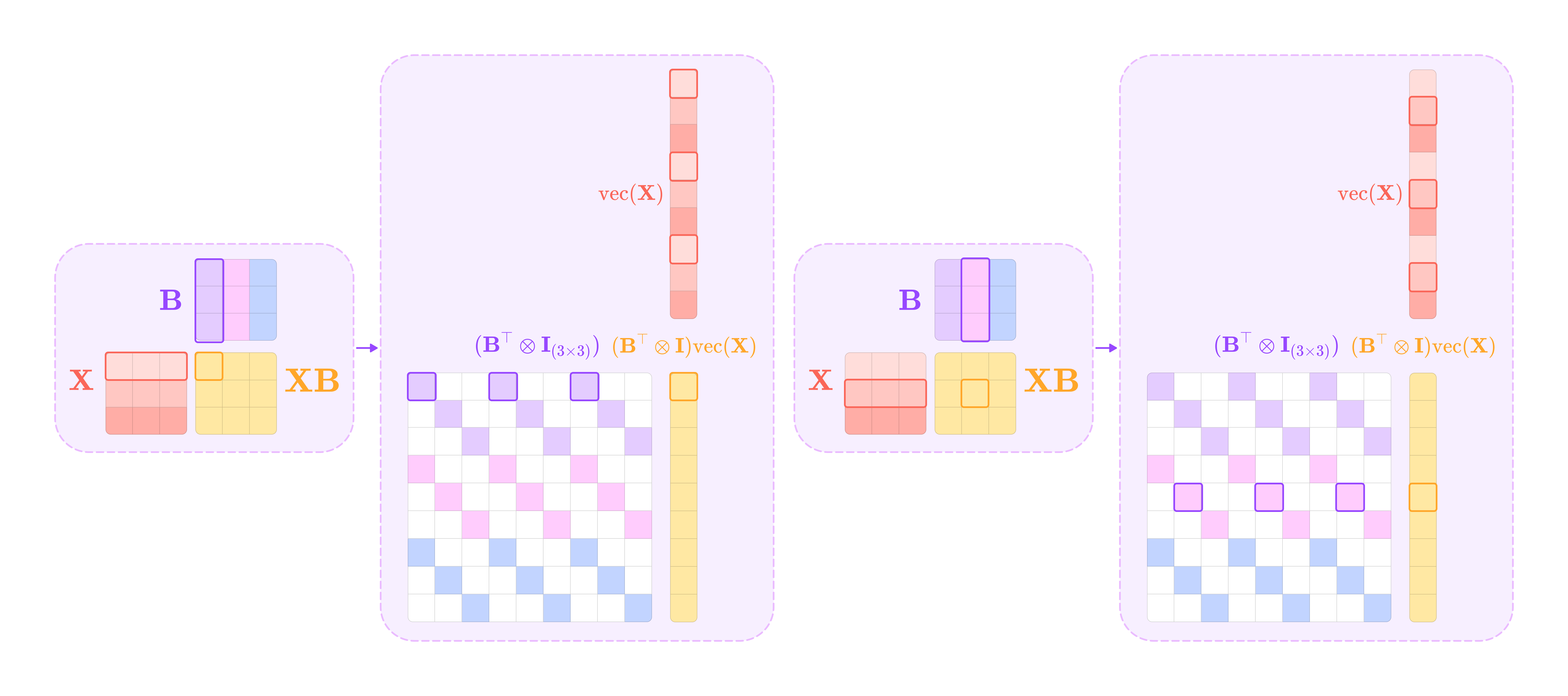
Making these substitutions allows us to isolate the vectorized matrix X:
This is in the form of the homogenous matrix-vector product Mx = 0, where we can solve for the vector x by finding the non-zero vectors in the null space of M. In the equation above, we can solve for the vectorized matrix X, by finding the null space of the following matrix:
In our case, we want to solve the following homogeneous equation:
Let’s break down how the type-J slice of the change-of-basis matrix Q transpose is computed in the code implementation:
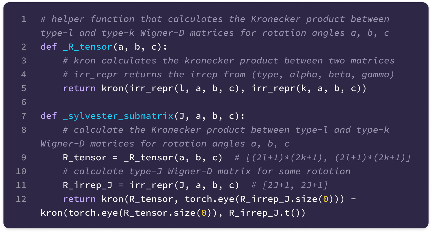
First, we calculate the type-l, type-k, and type-J Wigner-D matrices on randomly defined Euler angles alpha, beta, and gamma. For the type-l and type-k matrices, we take their Kronecker product, producing a (2l+1)(2k+1) x (2l+1)(2k+1) matrix. Note that the implementation of the kron function takes the second matrix in the Kronecker product as the first input and the first matrix as the second input.
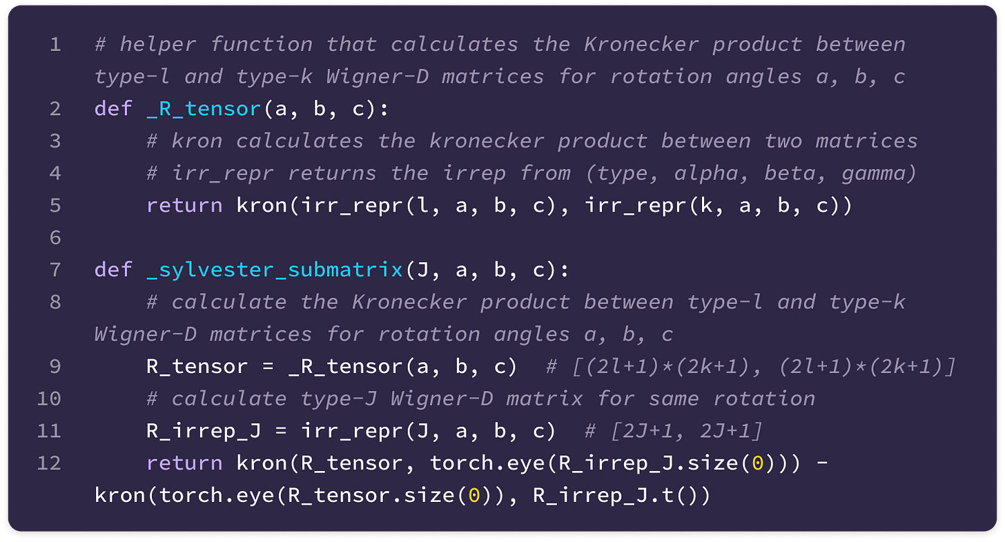
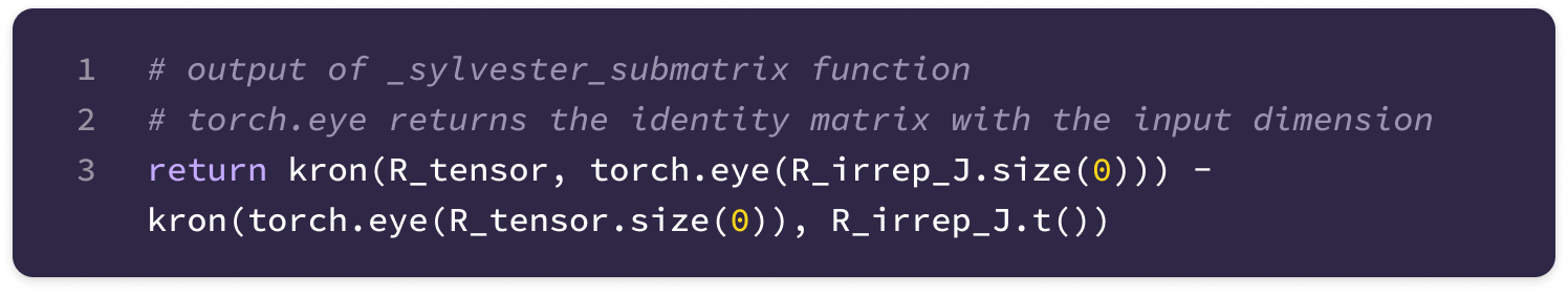
Now, we take the Kronecker product of the (2J+1) x (2J+1) identity matrix with the (2l+1)(2k+1) x (2l+1)(2k+1) Kronecker product of types l and k Wigner-D matrices and subtract the Kronecker product between the (2J+1) x (2J+1) transposed type-J Wigner-D matrix and the (2l+1)(2k+1) x (2l+1)(2k+1) identity matrix.
The complementary dimensions of the identity matrices turn A and B into (2l+1)(2k+1)(2J+1) x (2l+1)(2k+1)(2J+1) matrices that can subtracted element-wise from each other and used to solve the Sylvester equation.
\((\mathbf{I}_{(2J+1)\times(2J+1)}\otimes (\mathbf{D}_k(g)\otimes\mathbf{D}_l(g)))-(\mathbf{D}_J(g)^{\top}\otimes\mathbf{I}_{(2l+1)(2k+1)\times (2l+1)(2k+1)})\)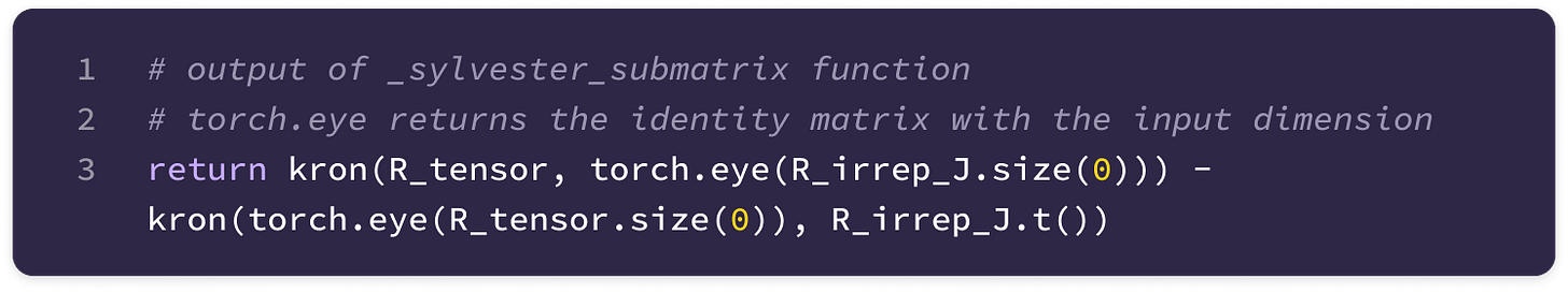
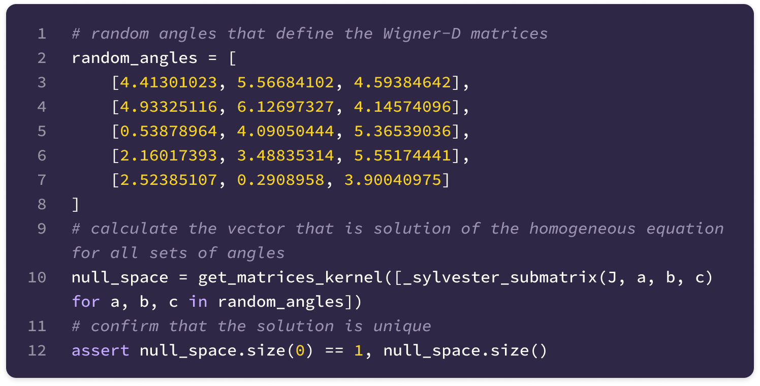
Next, we call the function defined in steps 1 and 2 to generate the Kronecker product matrix for five sets of random angles and calculate the vectors in the null space of all five matrices. Using multiple sets of random angles ensures the solution is unique and can be used as the change-of-basis Q across all rotations in SO(3).
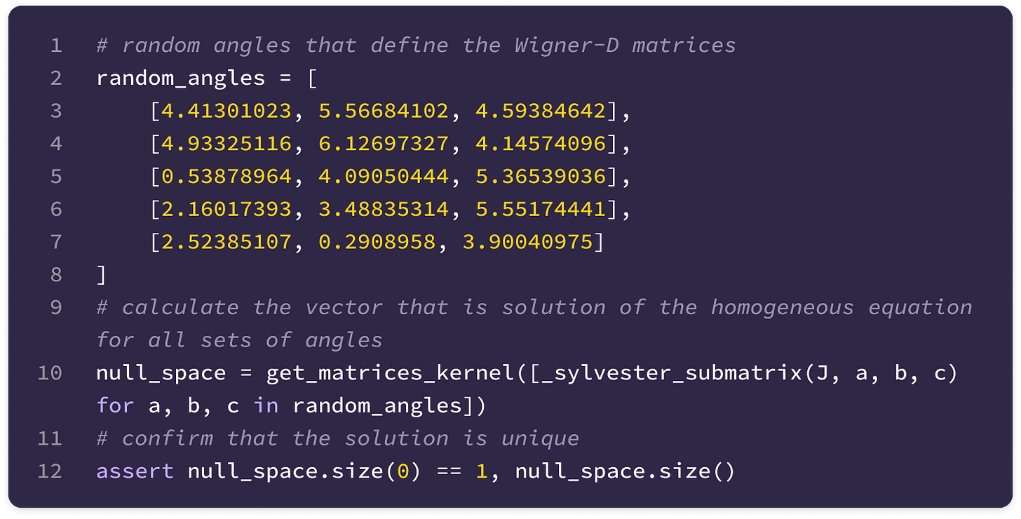
Finally, we reshape the vector into the matrix Q transpose with dimensions (2l+1)(2k+1) x (2J+1) and verify that it satisfies the homogeneous equation below for randomly generated angles.
\((\mathbf{D}_k(g)\otimes\mathbf{D}_l(g))\mathbf{Q}^{lk\top}_J-\mathbf{Q}^{lk\top}_J\mathbf{D}_J(g)=0\)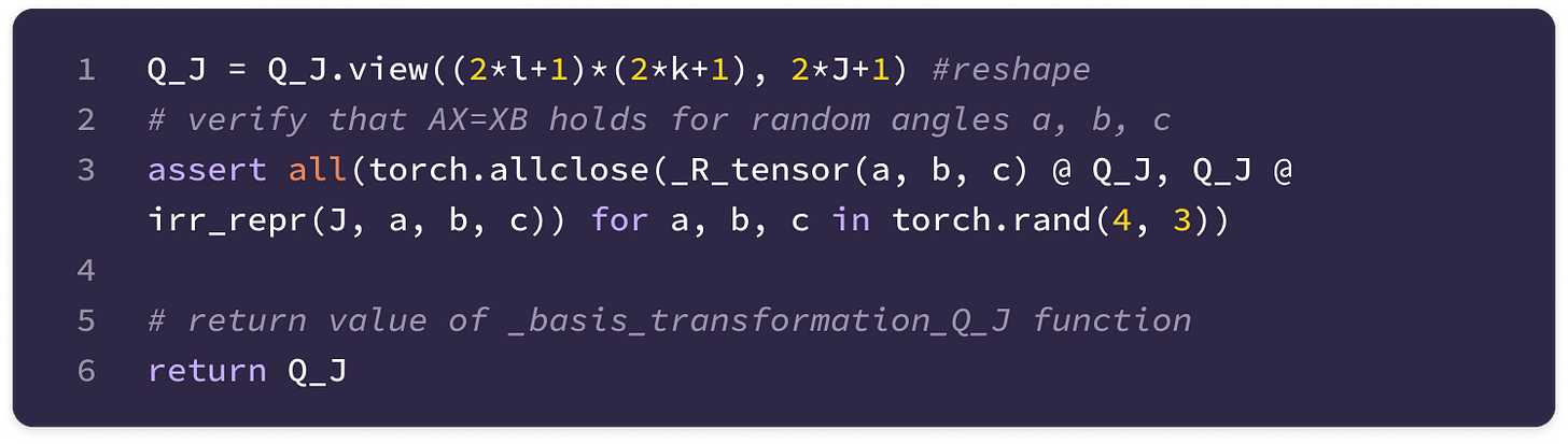
Now, we must compute the spherical harmonics projections of the angular unit displacement vector. Given that the spherical harmonic function must be computed for all 2J+1 values of m corresponding to all 2min(l,k)+1 values of J needed for all transformations between pairs of input and output degrees for every edge in the graph, the number of computations increases quickly with larger and more complex graphs.
To speed up computation, the SE(3)-Transformer precomputes the spherical harmonic projections for values of J up to double the maximum feature degree (since J has a maximum value of k + l) for every edge in the graph using recursive relations of the associated Legendre polynomials (ALPs).
The ALP term of the spherical harmonic equation is the most computationally intensive and needs to be recomputed for every edge of the graph since it is dependent on x=cos(θ), where θ is the polar angle of the angular unit vector. Using recursive relations, we only need to compute the ALP for boundary values of m=J, and the remaining polynomials can be derived from recursively combining the previously computed polynomials and storing them to compute the next set of polynomials.
The recursive computation of all non-zero ALPs for all values of J and m involves only three equations applied in the following sequence of steps:
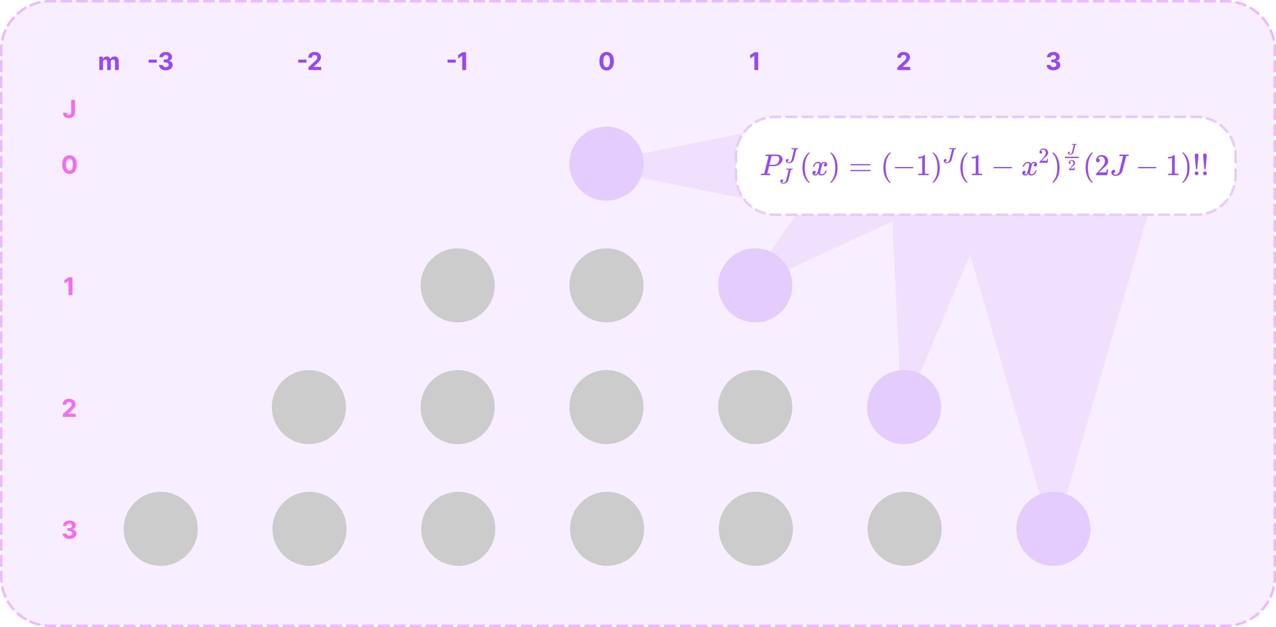
When m=J, which is the maximum value of m where the ALP is non-zero, we can calculate it directly with the following equation:
\(P^J_J(x)=(-1)^J(1-x^2)^\frac{J}{2}(2J-1)!!\tag{$m=J$}\)where x!! is the semi-factorial given by:
\(x!! = x(x-2)(x-4)\dots\)Notice that the Legendre polynomial in this equation is a constant since taking the mth derivative reduces the degree to 1.
Calculating the boundary ALPs for m=J. (Source: Alchemy Bio) Then, we can compute the polynomials for when m=J-1 from the polynomials stored from step 1 using the following recursive relation:
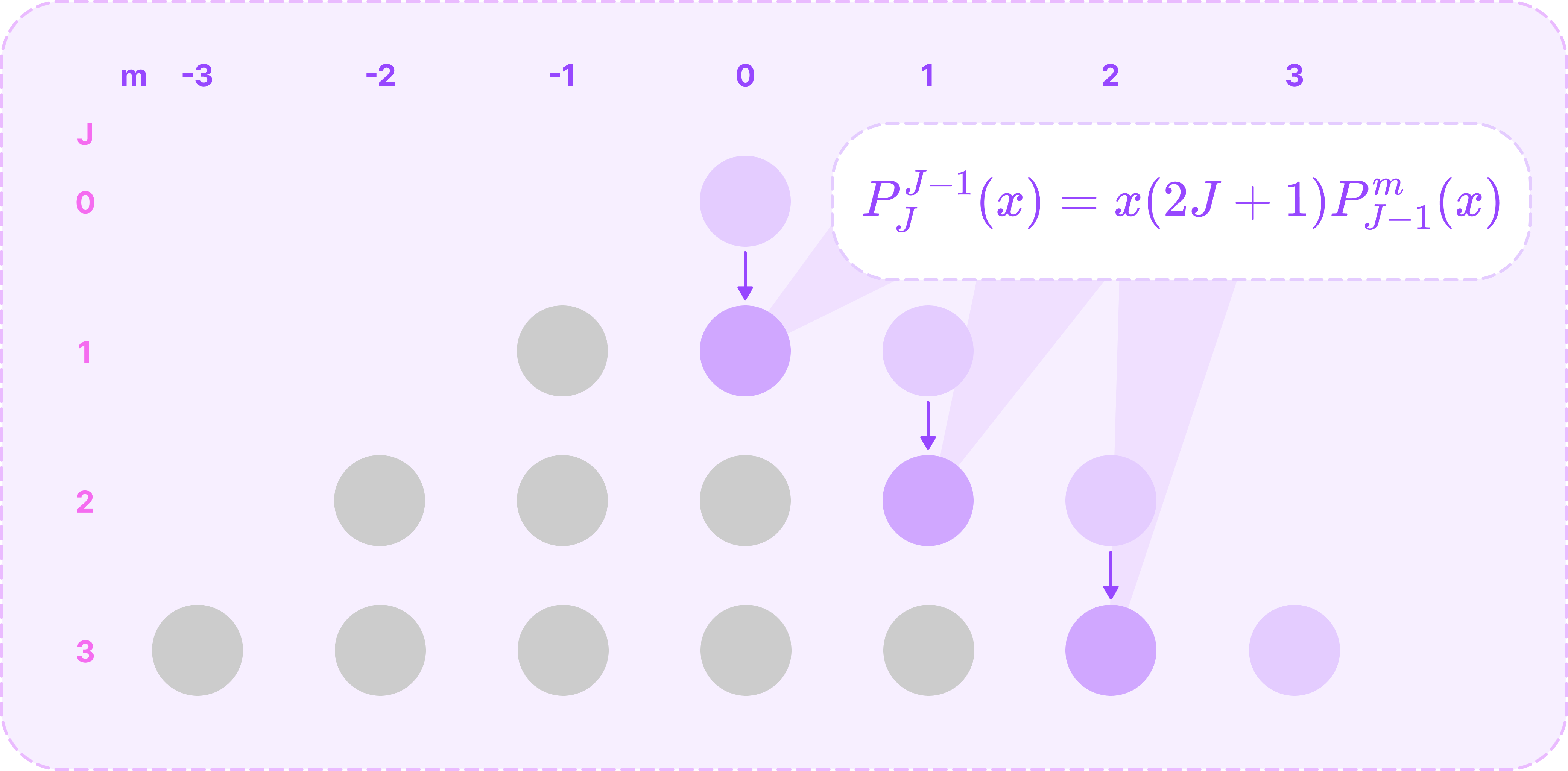
\(P^{J-1}_{J}(x)=x(2J+1)P^m_{J-1}(x)\tag{$m=J-1$}\)
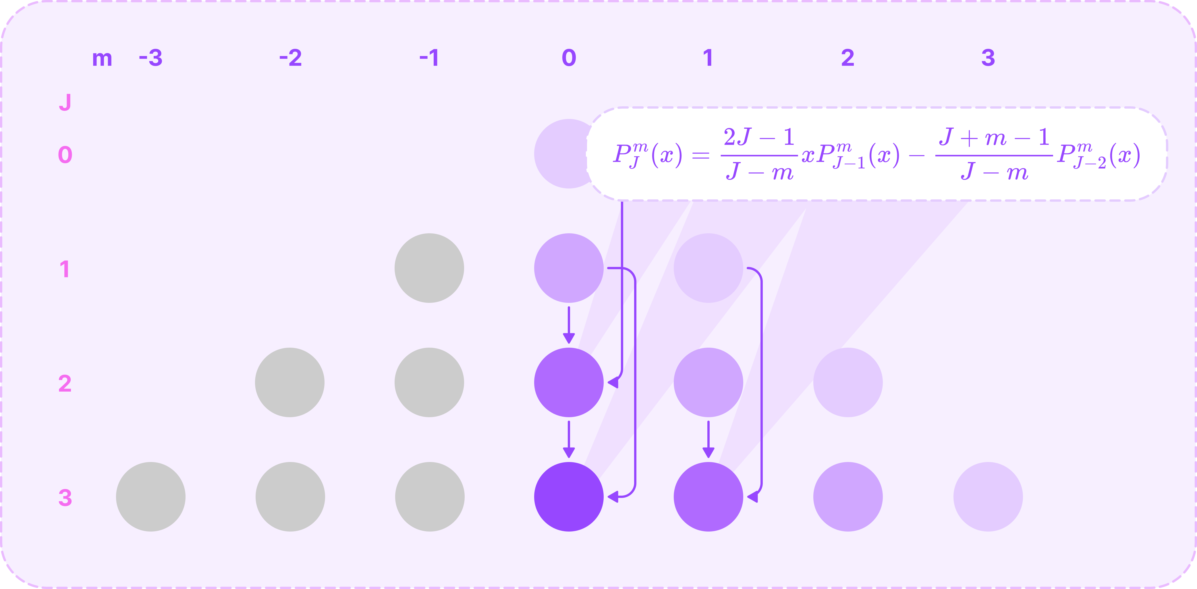
Calculating the ALPs for m=J-1 from the boundary ALPs. (Source: Alchemy Bio) For the remaining ALPs with non-negative values of m, we can compute it recursively from the two preceding ALPs with order m and degrees J-1 and J-2 using the recursive relation below:
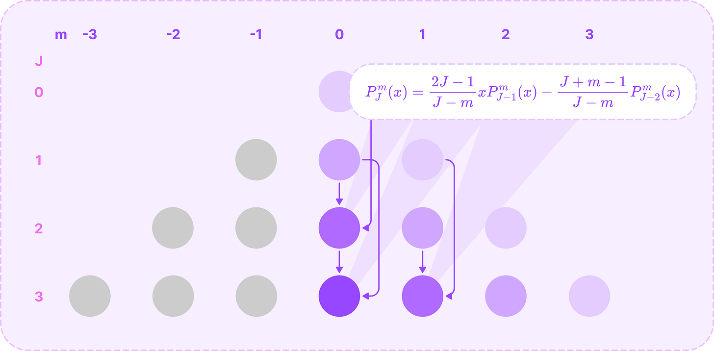
\(P^m_{J}(x)=\frac{2J-1}{J-m}xP^m_{J-1}(x)-{\frac{J+m-1}{J-m}P^m_{J-2}(x)}\tag{$m\geq 0$}\)Notice that the recursive relation for step 2 is just the first term of this equation, simplified for m=J-1.
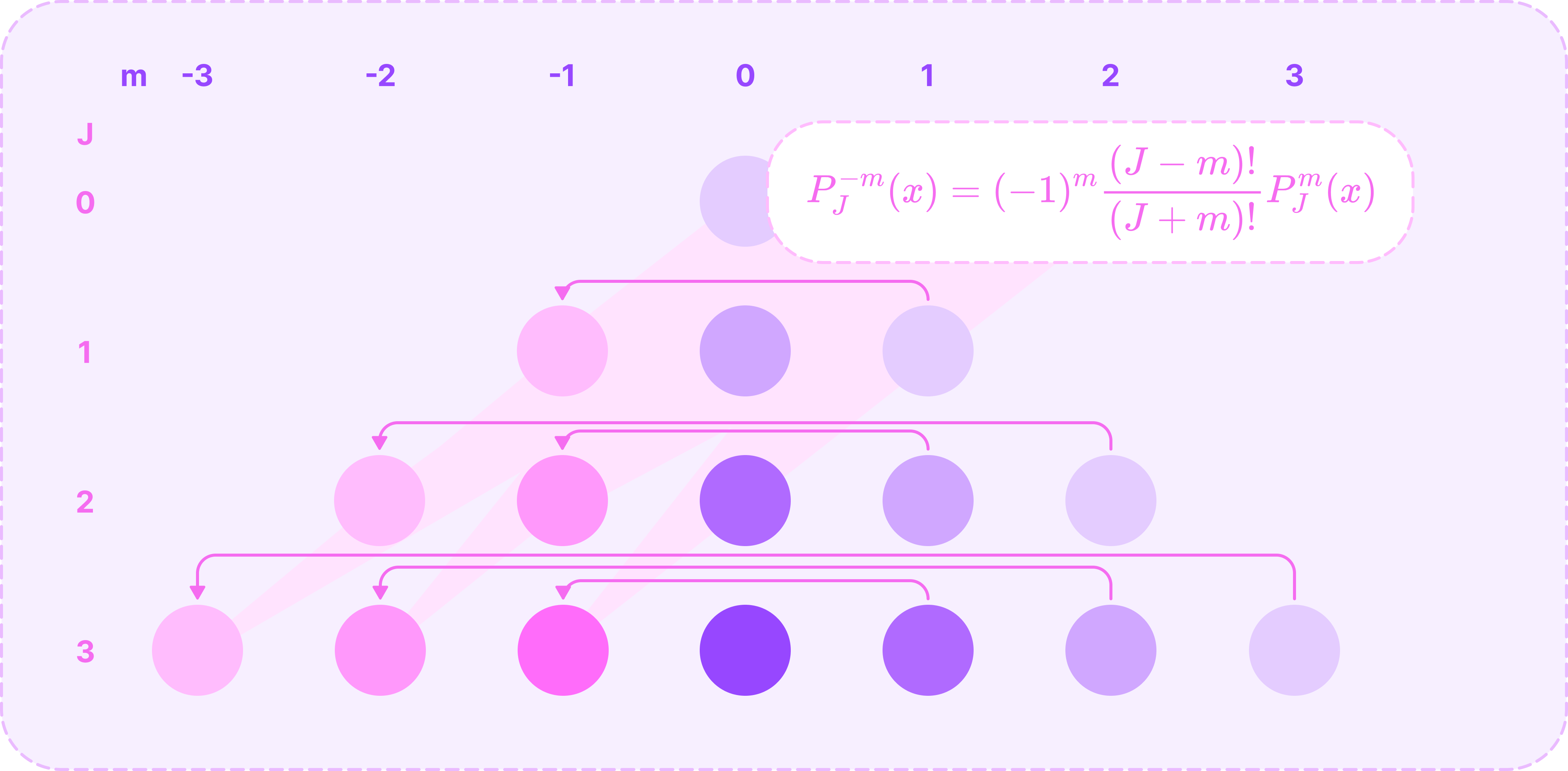
Calculating all ALPs for non-negative m with previously computed ALPs. (Source: Alchemy Bio) Finally, we can compute the ALPs for all negative values of m from the ALP of its positive counterpart using the following relationship:
\(P^{-m}_J(x)=(-1)^m\frac{(J-m)!}{(J+m)!}P^m_J(x)\)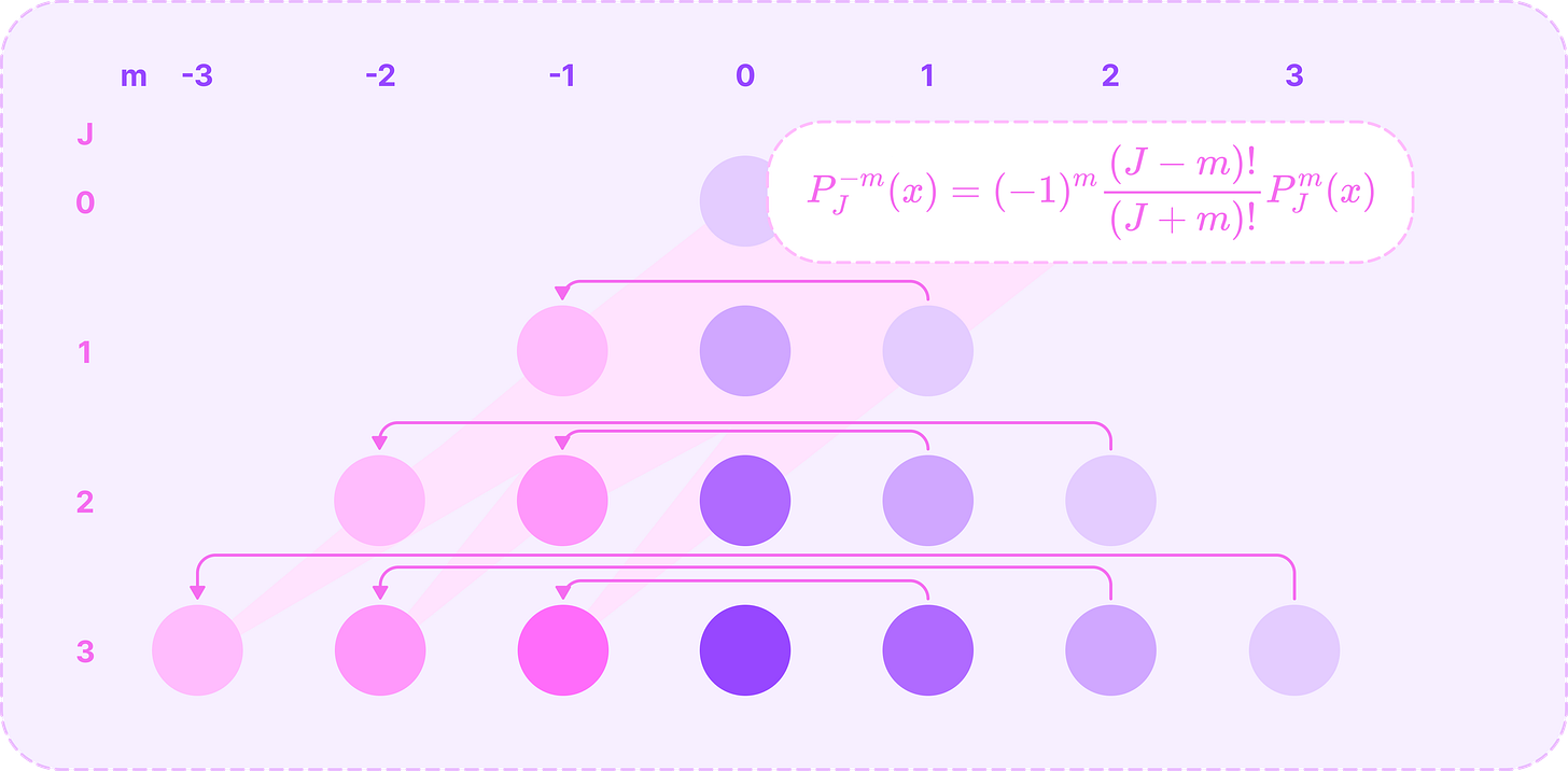
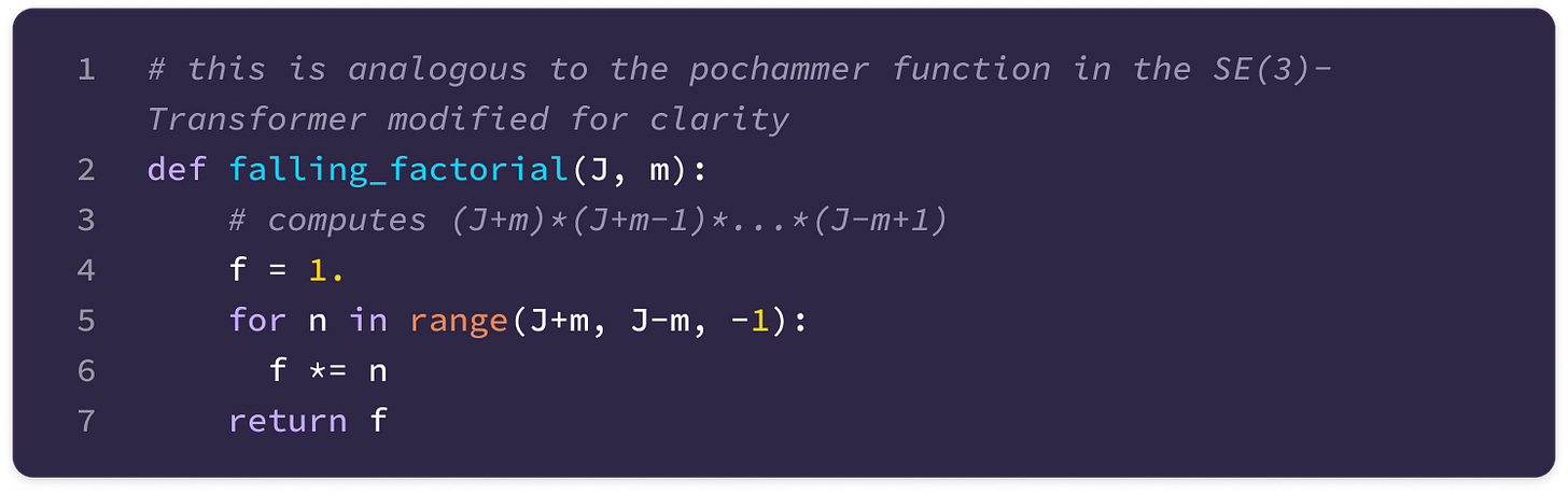
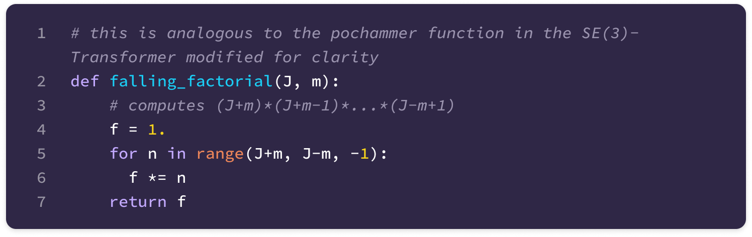
Calculating all ALPs for negative orders m using its positive counterpart. (Source: Alchemy Bio) In this equation, the fraction term can be written in terms of the inverse of a falling factorial from (J+m) to (J-m+1):
\(\begin{align}\frac{(J-m)!}{(J+m)!}&=\frac{\cancel{(J-m)}\cdot \cancel{(J-m-1)}\cdot \ldots \cdot \cancel{1}}{(J+m)\cdot(J+m-1)\cdot \ldots\cdot\cancel{(J-m)}\cdot\cancel{(J-m-1)}\cdot \ldots\cdot \cancel{1}}\nonumber\\&=\frac{1}{(J+m)\cdot (J+m-1)\cdot\ldots \cdot(J-m+1)}\nonumber\end{align}\)We can calculate the falling factorial for a given value of J and m using the following helper function:
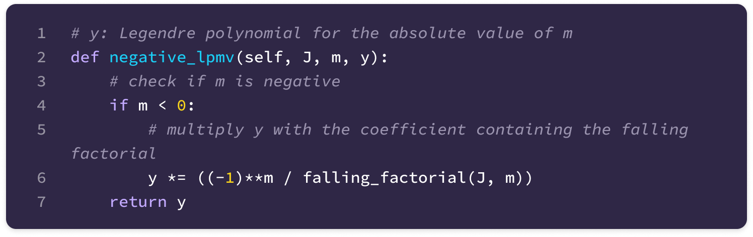
If m is negative, the function below takes the polynomial for the absolute value of m and returns the polynomial scaled by the negative coefficient:

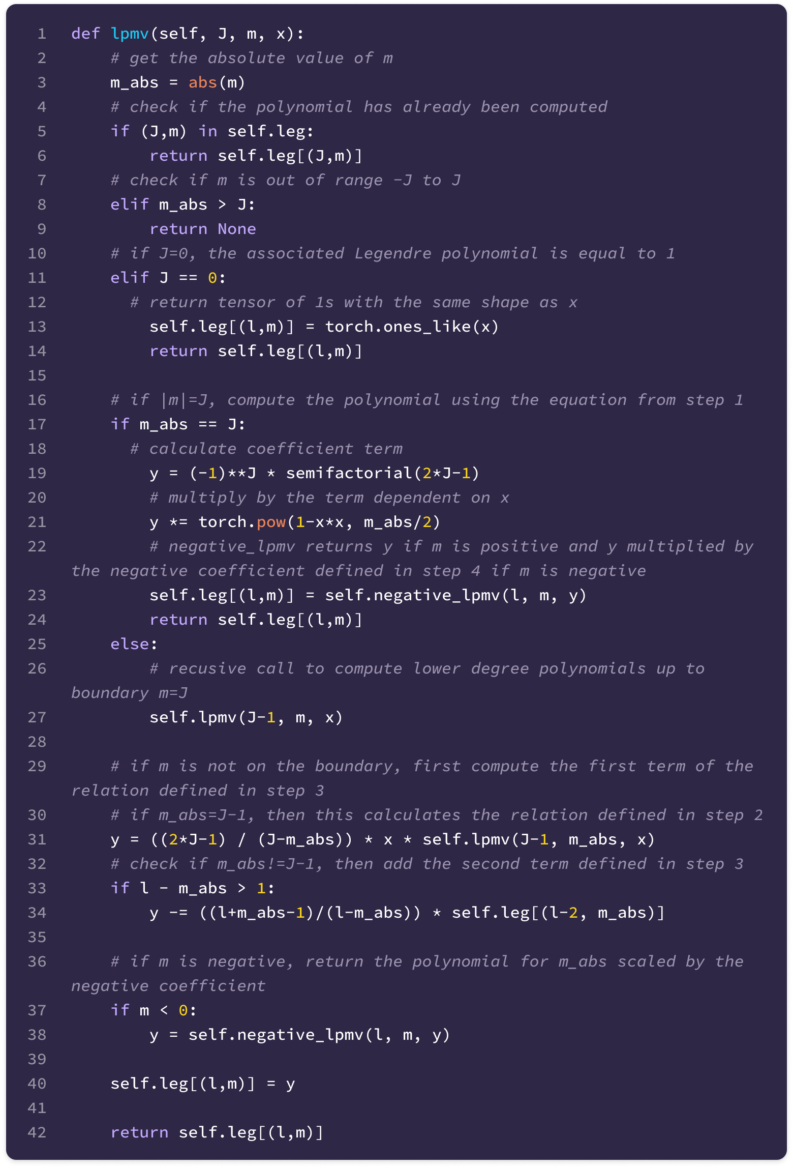
Now that we understand how the recursive relations work, we can implement the code that returns the ALP for a given m and J either by applying the recursive relations using previously stored ALPs or making a recursive call to compute the ALP for m and J-1 until the boundary where m=J:
After computing the ALP, we can calculate the real spherical harmonics from the associated Legendre polynomials with the following equations, depending on the sign of m:
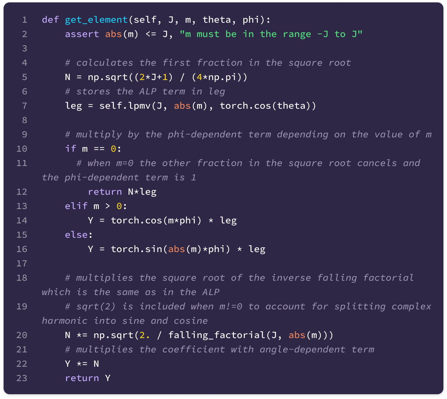
This can be converted into the following function that returns the spherical harmonic given values of J, m, θ (theta), and φ (phi):
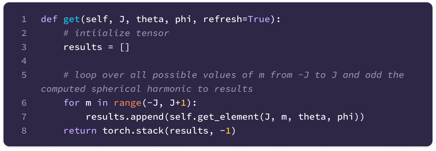
Now, we can generate the tensor of spherical harmonics for all values of m corresponding to a given J, which is a type-J spherical tensor:
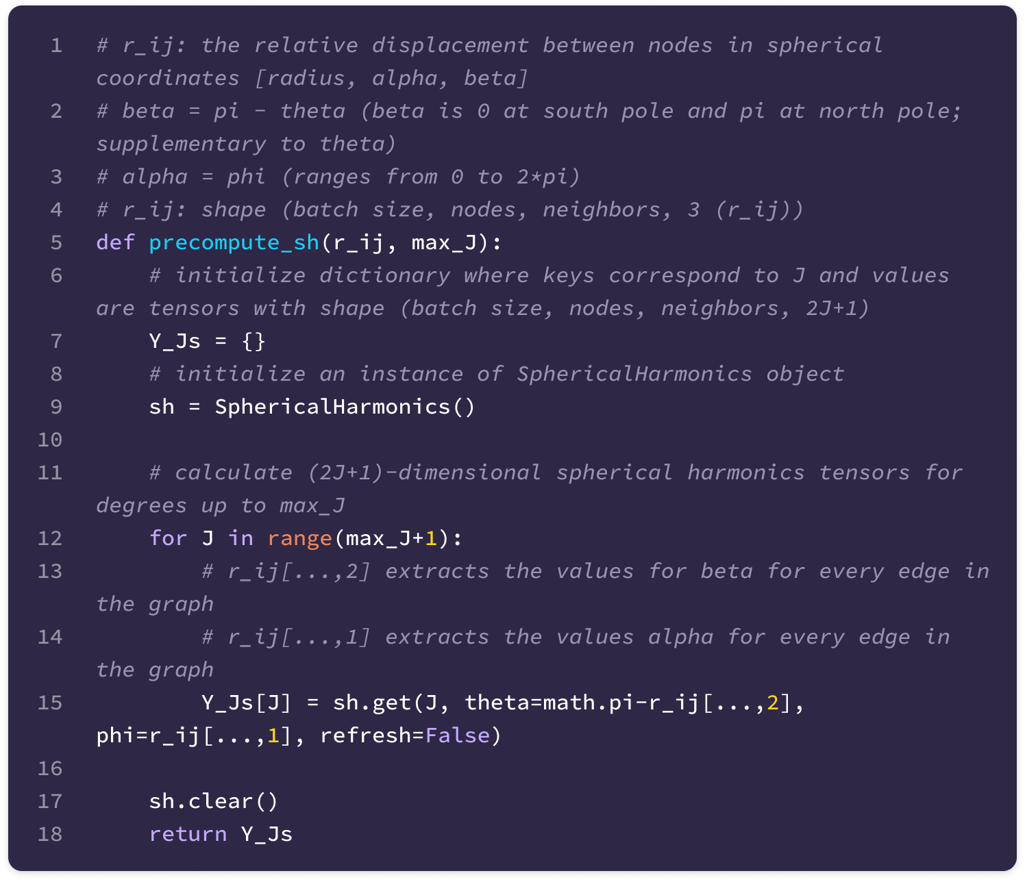
The function below is called to calculate the spherical harmonics given the relative displacement vector between nodes in spherical coordinates, using the angle conventions from the implementation of the 3D steerable CNN where each edge is represented by the radius, beta (angle from south pole), and alpha (same as phi in spherical harmonics):
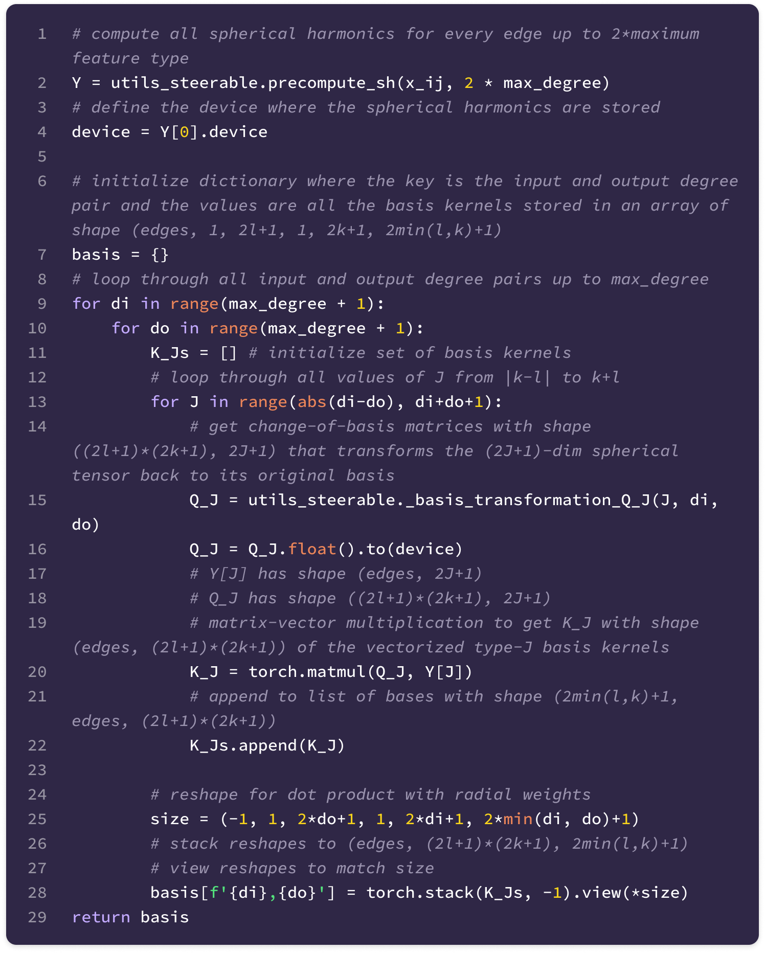
Finally, the basis kernels for all values of J up to a maximum feature degree are computed and stored so that the kernels across every layer in the model transforming from type-l to type-k features can be derived simply by taking a linear combination of stored basis kernels for J from |k-l| to k+l.
The shape of the set of basis kernels for a given transformation between types k and l is (1, 2l+1, 1, 2k+1, num bases) where the singleton dimensions will be broadcasted into the number of input and output channels when taking the weighted sum to generate a unique kernel that transforms from a specific type-k input channel to a specific type-l output channel.
Constructing the Radial Function
We can construct equivariant kernels by scaling the basis kernels with learned radial functions that transform the radial distance between nodes a set of weights. This function is a feed-forward network (FFN) that is effective in learning complex dependencies between the basis kernels and the distance between nodes.
Since each basis kernel represents a unique function that changes with a defined pattern on the unit sphere (defined by the spherical harmonic), we need to incorporate learnable parameters when constructing the equivariant kernels so that they can learn to detect specific feature motifs represented by distinct weighted combinations of the basis kernels.
The radial function not only allows us to incorporate distance dependence, which contributes to the strength of relationships between nodes, but it also allows the model to learn more complex dependencies on the node and edge features through backpropagation.
To construct the kernel that transforms type-k to type-l features, we define a radial function that takes the scalar distance as input and returns a weight for each basis kernel for values of J from |k-l| to |k+l|. For multi-channel features, the radial function not only generates a unique weight for each value of J but also for every input-to-output channel pair. This means that the output of the function is a (num_bases)*(input_channels)*(output_channels)-dimensional vector of weights.
We can denote a single weight produced by the function with the following notation:
Since rotating a vector does not change its length, the radial distance is SO(3)-invariant. This means the output of the radial function is invariant to rotations of the input graph for any function definition:
Thus, we define the radial function as a feed-forward network (FFN) with multiple linear layers interspersed with nonlinear activation functions to maximize the model’s ability to learn and detect complex feature motifs. The linear layers of an FFN can transform a vector from one dimension to another via multiplication with a (output dimension) x (input dimension) matrix of learnable weights and the addition of a bias vector with the same dimension as the output. Linear layers are followed by nonlinear activation functions like ReLU or LeakyReLU that capture more complex dependencies across weights.
A new network is constructed for every ordered pair (k, l) of input and output feature types and every equivariant layer or type of embedding (attention layers have different networks for generating key and value embeddings). Each network is used across all nodes in the graph.
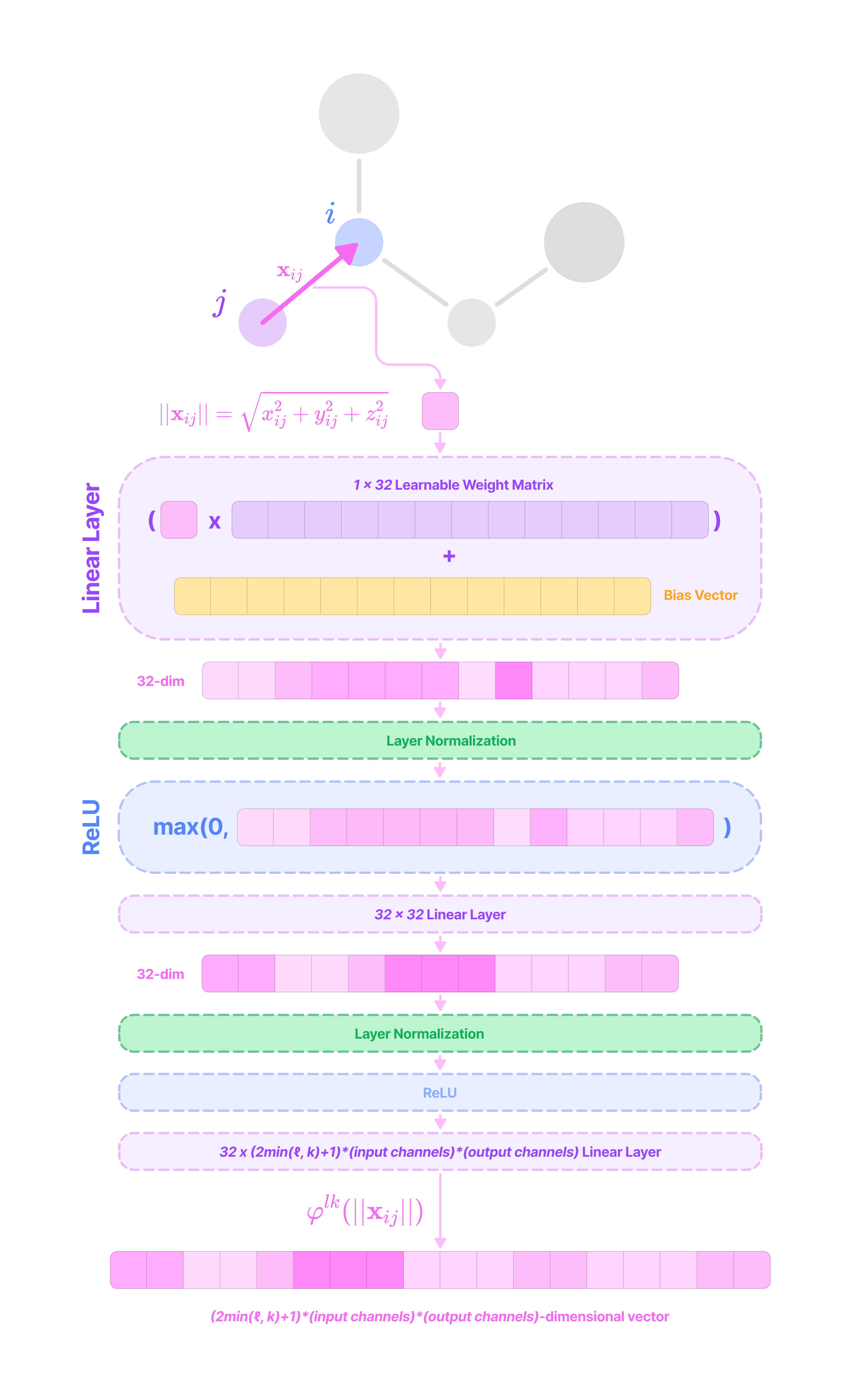
The FFN used in the SE(3)-Transformer consists of the following layers:
The first linear layer transforms the input into a 32-dimensional vector by multiplication with a 32 x 1 learnable weight matrix and addition with a 32-dimensional bias vector.
\(\mathbf{W}_1||\mathbf{x}_{ij}|| + \mathbf{b}_1\tag{$\mathbf{W}_1\in \mathbb{R}^{32\times 1}$}\)A layer normalization step transforms the mean to 0 and the variance to 1 across the values in the 32-dimensional vector.
A non-linear ReLU activation function is applied element-wise. For each element, the ReLU function outputs 0 for negative values or itself for positive values.
\(\mathbf{x}'=\max\left(0,\text{LayerNorm}(\mathbf{W}_1||\mathbf{x}_{ij}|| + \mathbf{b}_1)\right)\)Another FFN block with a linear layer (hidden dimension of 32), normalization step, and ReLU activation function is applied.
A final linear layer transforms the 32-dimensional vector output of the second block into a (2min(l, k)+1)(mi)(mo)-dimensional vector by multiplication with a (2min(l, k)+1)(mi)(mo) x 32 matrix of learnable weights and addition with a (2min(l, k)+1)(mi)(mo)-dimensional bias vector.
\(\begin{align}\varphi^{lk}(||\mathbf{x}_{ij}||)=\mathbf{W}\mathbf{x}'' + \mathbf{b}_2\;\;\;\;(\mathbf{W}_2\in \mathbb{R}^{32\times (2min(l,k)+1)(c_k)(c_l)})\nonumber\end{align}\)
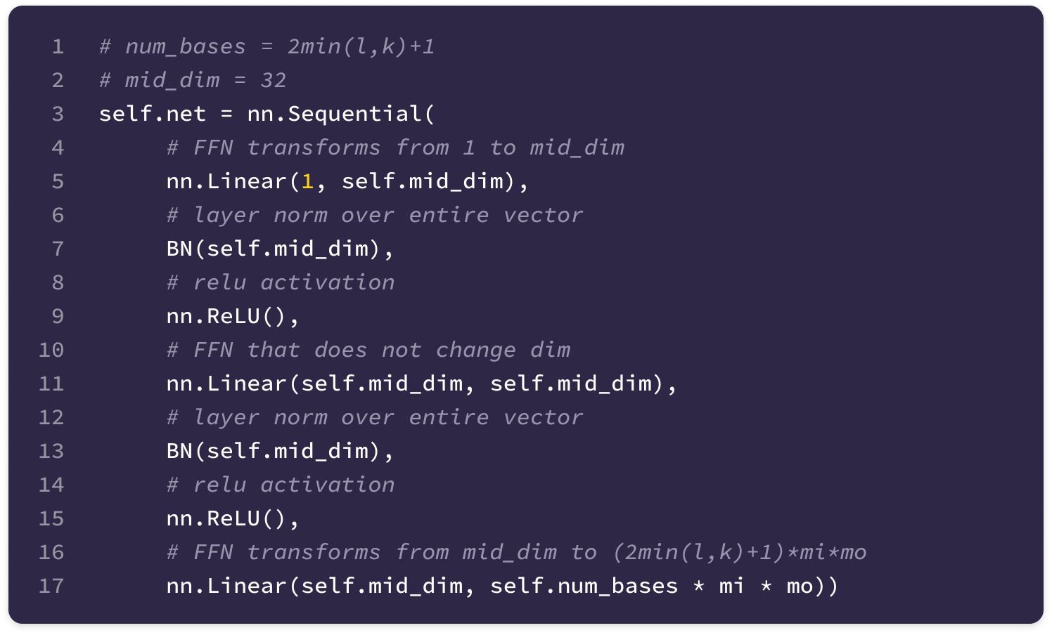
The FNN can be constructed in PyTorch with the following code:
Then, we can generate the radial weights for a given pair of input and output types k, l:
Mechanism of the Equivariant Kernel
To grasp how the equivariant kernel is able to capture high-frequency rotationally-symmetric patterns in a single matrix-vector multiplication step, let’s break down how to interpret the mechanism of the kernel in terms of tensor products.
Given that each input-to-output channel pair has a unique radial weight, from now on, we will denote the kernel that transforms the type-k feature at channel c_k in node j for message passing to the type-l feature at channel c_l in node i as:
The weighted kernel acts as an aggregated function that takes multiple tensor products between the type-k input feature tensor and all the type-J projections of the displacement vector.
Intuitively, we can think of the kernel transformation as performing the following operations:
Extracting the type-l tensor component of the tensor product between the type-k feature tensor with the type-J spherical tensor projection of the displacement vector via the Clebsch-Gordan coefficients. Each dimension (indexed by the magnetic quantum number m_l) of the type-l tensor component can be written as:
\((\mathbf{Y}^{(J)}(\hat{\mathbf{x}}_{ij})\otimes\mathbf{f}^{k}_{\text{in,}j,c_k})^{(l)}_{m_l}=\sum_{m=-J}^J\sum_{m_k=-k}^kC^{(l, m_l)}_{(J, m)(k, m_k)}Y^{(J)}_{m}f^{(k)}_{m_k}\)We can write the full type-l tensor as a (2l + 1)-dimensional vector by concatenating all dimensions indexed by m from -l to l :
\((\mathbf{Y}^{(J)}(\hat{\mathbf{x}}_{ij})\otimes\mathbf{f}^{k}_{\text{in,}j,c_k})^{(l)}=\begin{bmatrix}(\mathbf{Y}^{(J)}(\hat{\mathbf{x}}_{ij})\otimes\mathbf{f}^{k}_{\text{in,}j,c_k})^{(l)}_{-l} \\\\ (\mathbf{Y}^{(J)}(\hat{\mathbf{x}}_{ij})\otimes\mathbf{f}^{k}_{\text{in,}j,c_k})^{(l)}_{-l+1} \\ \vdots \\(\mathbf{Y}^{(J)}(\hat{\mathbf{x}}_{ij})\otimes\mathbf{f}^{k}_{\text{in,}j,c_k})^{(l)}_{l} \end{bmatrix}\)Scaling the type-l tensor component by the weight calculated by a learnable function on the radial component of the displacement vector.
\(\varphi^{lk}_{(J,c_l,c_k)}(||\mathbf{x}_{ij}||)(\mathbf{Y}^{(J)}(\hat{\mathbf{x}}_{ij})\otimes\mathbf{f}^{k}_{\text{in,}j,c_k})^{(l)}\)Repeating Steps 1 and 2 for all types-J projections of the angular unit vector ranging from |k - l| to |k + l| and scaling the type-l output by a unique learnable weight. Then, taking the sum of all the weighted type-l components of the tensor products to get the output type-l message for channel c_l from the type-k feature at channel c_k:
\(\mathbf{W}^{lk}_{(c_l,c_k)}(\mathbf{x}_{ij})\mathbf{f}^k_{\text{in,}j,c_k}=\sum_{J=|k-l|}^{k+l}\varphi^{lk}_{(J,c_l,c_k)}(||\mathbf{x}_{ij}||)(\mathbf{Y}^{(J)}(\hat{\mathbf{x}}_{ij})\otimes\mathbf{f}^k_{\text{in,}j,c_k})^{(l)}\)
Instead of performing all these steps and taking the tensor product with every type-J projection, the equivariant kernel aggregates all of these operations into a single kernel matrix-vector multiplication step.
Rules of Equivariant Layers
Now, let’s quickly solidify some general rules when constructing equivariant layers:
To transform between spherical tensors of different types, we must take the tensor product, which generates a higher-dimensional tensor that can be decomposed into its spherical tensor components. Then, we can extract the target feature type from the decomposition to combine it with other tensors of the same type. This process can be condensed into a single matrix-vector multiplication step with an equivariant kernel that combines spherical harmonics and Clebsch-Gordan coefficients such that it satisfies the kernel constraint.
Applying non-linear functions element-wise to spherical tensors with degrees greater than 0 breaks equivariance. To introduce non-linearities, we can incorporate nonlinearities into learnable functions that transform scalar or higher-dimensional spherical tensors into scalar weights that can be multiplied across all elements of a spherical tensor.
All group representations including Wigner-D matrices are linear transformations from a tensor space to itself that act exclusively on a type of spherical tensor. This means that Wigner-D matrices preserve addition and scalar multiplication of tensors with the same type. This means we can combine multiple features across channels of the same type by taking weighted sums.
\(\mathbf{D}_l(g)(a\mathbf{s}^l+b\mathbf{t}^l)=a\mathbf{D}_l(g)\mathbf{s}^l+b\mathbf{D}_l(g)\mathbf{t}^l\tag{$a,b\in \mathbb{R}$}\)This makes intuitive sense when considering scaling and adding vectors in 3D space. Rotating the sum of two 3D vectors is equivalent to rotating the two vectors and taking their sum. This generalizes to higher-degree spherical tensors, since by definition, tensors of the same type transform under the same set of irreps that preserve lengths and angles between tensors.
Since graphs are considered unordered sets of nodes, operators used to aggregate messages must be permutation-invariant such that the order in which the messages are aggregated does not change the output. The operators must also be equivariant to rotation, which includes taking the weighted sum or average (which is just the sum scaled by the fraction with the total number of messages in the denominator) of messages of the same type.
With these rules in mind, let’s break down how to build one of the first fully SO(3)-equivariant modules for geometric graphs: the Tensor Field Network (TFN).
Tensor Field Network Module
The tensor field network (TFN) introduced by Thomas et al. is an SE(3)-equivariant model that takes a point cloud and applies an equivariant kernel that outputs a geometric tensor at every point in space (defintiion of a tensor field) using spherical harmonics and radial weights. The TFN layer in the SE(3)-Transformer is used to reduce high-degree attention embeddings into lower-degree tensors before generating a prediction.
The TFN layer generates a message for every channel of every feature type for every node in the graph with the equation below, which will be the focus of this section:
This message generated above is used to update the type-l feature at channel c_l at node i:
Equivariant Message-Passing
Since we have already described the function of the equivariant kernel, this section will focus on breaking down how the messages are aggregated and implementing it in code.
For every node in the graph, the TFN layer updates the input feature tensor with an updated output feature tensor generated equivariantly from the input features of adjacent nodes. This process involves the following steps:
First, we construct a new radial network for all k → l transformations with an output dimension of (2min(l,k)+1)*(type-k input channels, mi)*(type-l output channels, mo) which will be used to calculate unique radial weights for every basis kernel and every possible path from a type-k input channel to a type-l output channel.
The radial distance corresponding to every edge is fed into the (k, l) radial function to obtain an array of radial weights with shape (mo, 1, mi, 1, num bases). We will discuss how other scalar edge features can be incorporated in this step later.
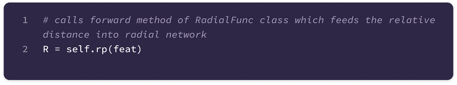
For a given edge, we obtain the kernel of the transformation of features from an input type-k channel c_k to an output type-l channel c_l by taking a weighted sum of all basis kernels scaled by their corresponding radial weight.
\(\mathbf{W}^{lk}_{(c_l,c_k)}(||\mathbf{x}_{ij}||)=\sum_{J=|k-l|}^{k+l}\varphi^{lk}_{(J,c_l,c_k)}(||\mathbf{x}_{ij}||)\mathbf{W}^{lk}_{J}(||\mathbf{x}_{ij}||)\)In the code implementation, the singleton dimensions of the array of radial weights with shape (mo, 1, mi, num bases) and the array of basis kernels with shape (1, 2l+1, 1, 2k+1, num bases) are broadcasted to match each other, and the element-wise product of the two tensors is calculated. The resulting product is a set of weighted basis kernels for every input and output channel pair with shape (mo, 2l + 1, mi, 2k + 1, num_bases). Finally, we take the sum over the weighted basis kernels (last dimension) to get an array with shape (mo, 2l + 1, mi, 2k + 1), containing the final kernel for every pair of channels (c_l, c_k).
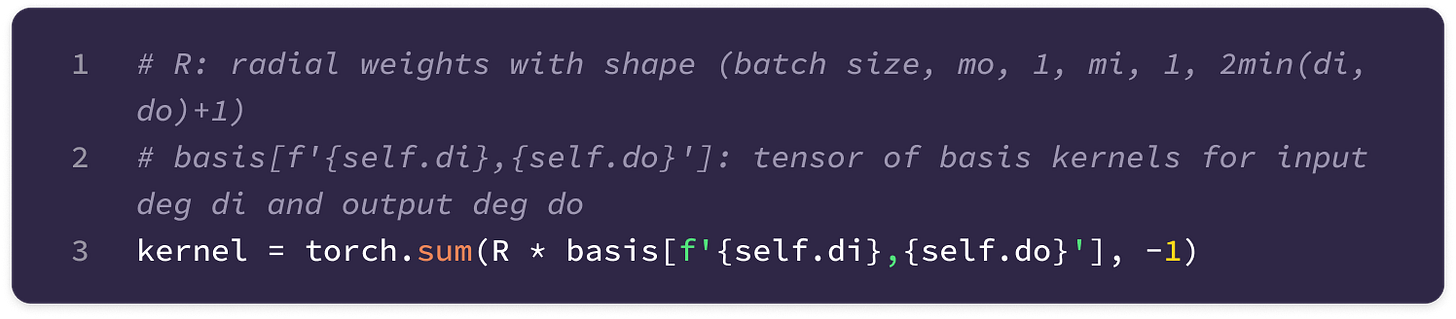
The kernel array is reshaped to have dimensions (mo)*(2l + 1) x (mi)*(2k + 1), where each block of the matrix is the (2l + 1) x (2k + 1) kernel corresponding to the transformation from input channel c_k to output channel c_l, denoted by the subscript (c_l, c_k).
\(\mathbf{W}^{lk}(\mathbf{x}_{ij})=\begin{bmatrix}\mathbf{W}^{lk}_{(1,1)}&\mathbf{W}^{lk}_{(1,2)}&\dots&\mathbf{W}^{lk}_{(1,\text{mi})}\\\\\mathbf{W}^{lk}_{(2,1)}&\ddots&\dots &\vdots \\\\\vdots &\dots &\ddots& \vdots\\\\\mathbf{W}^{lk}_{(\text{mo},1)}&\dots &\dots &\mathbf{W}^{lk}_{(\text{mo},\text{mi})}\end{bmatrix}_{(\text{mo}*(2l+1))\times(\text{mi}*(2k+1))}\)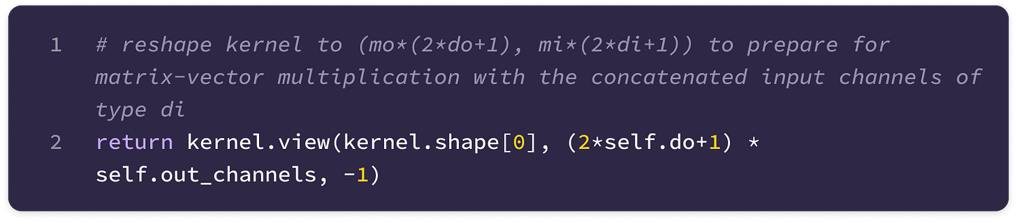
Now we calculate and store a kernel for every k → l transformation by looping through all (multiplicity, degree) tuples in the input and output fiber structures. The code for generating the kernel is implemented in the PairwiseConv class.
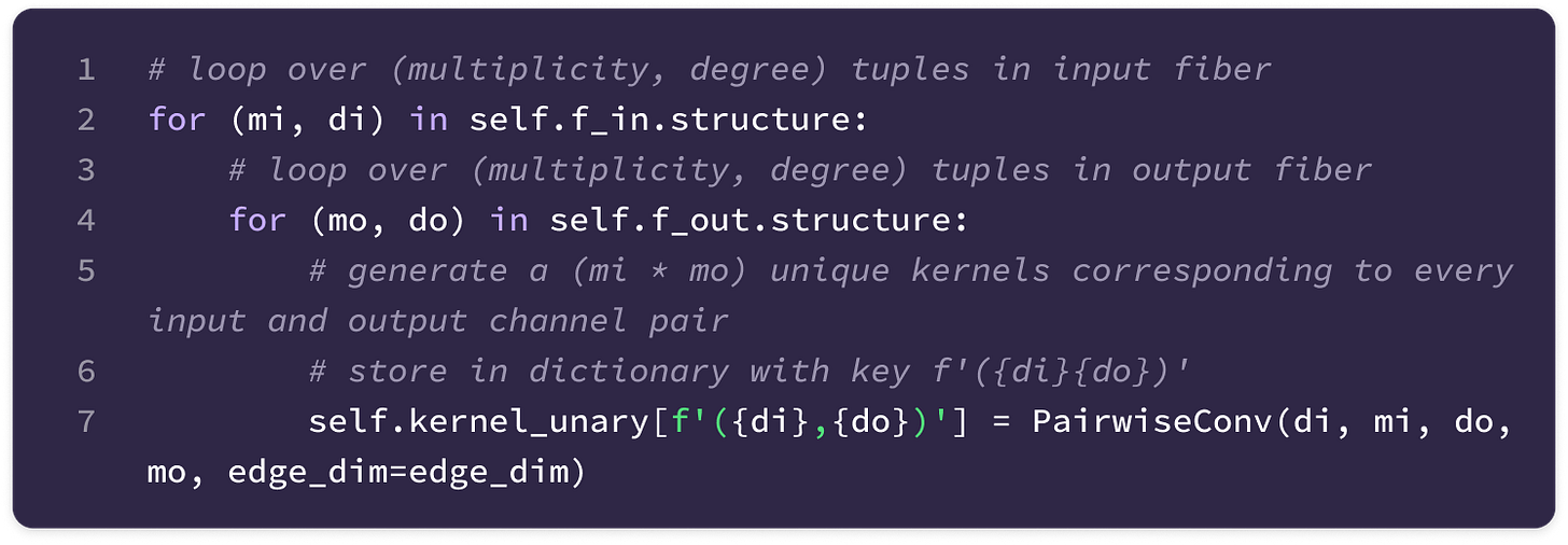
For every feature type in the output fiber, we can compute the message for a single type-l output channel c_l at the center node i from all the features at node j by:
Transforming the type-k input channel c_k into a type-l message by matrix multiplication with the uniquely defined kernel for output channel c_l
Taking the sum over channel c_l messages from all type-k input channels
Iterating for all feature types k defined in the input fiber and adding the type-l message from type-k input channels to the total type-l message with each iteration.
\(\underbrace{ \sum_{k \geq 0} \underbrace{ \sum_{c_k} \underbrace{ \mathbf{W}^{lk}_{(c_l,c_k)}(\mathbf{x}_{ij}) \mathbf{f}^k_{\text{in},j,c_k} }_{\text{(a) channels }c_k\to c_l\text{ message}} }_{\text{(b) message from type-}k\text{ input channels}}}_{\text{(c) type-}l\text{ channel }c_l\text{ message from node }j}\)In the code implementation, the messages for all type-l channels from a single input type k are calculated in parallel with a single matrix-vector multiplication step by concatenating all the type-k input features into a (mi)*(2k+1)-dimensional vector and multiplying it with the (mo)*(2l + 1) x (mi)*(2k + 1) block kernel defined above. The output of the kernel contains the messages for each type-l output channel stacked in a single (mo)*(2l+1)-dimensional vector, which is then summed together with the messages from each input degree k.
\(\underbrace{\sum_{k\geq0}\underbrace{\mathbf{W}^{lk}(\mathbf{x}_{ij})\bigoplus_{c_k}\mathbf{f}^k_{\text{in},j,c_k}}_{\text{message from type-}k\text{ input channels}}}_{\text{direct sum of type-}l\text{ messages from node }j}\)The code implementation calculates the type-l messages for every edge in the graph in parallel and reshapes the vectorized output messages into an array with shape (edges, mo, 2l+1).
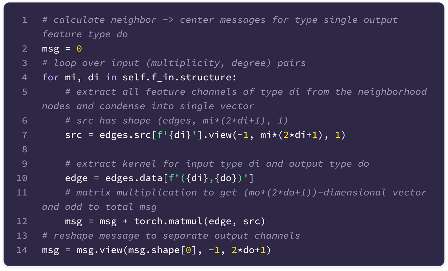
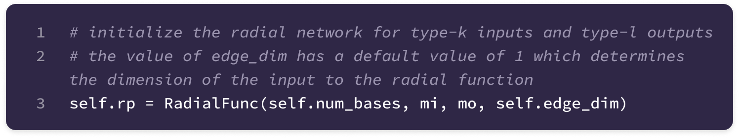
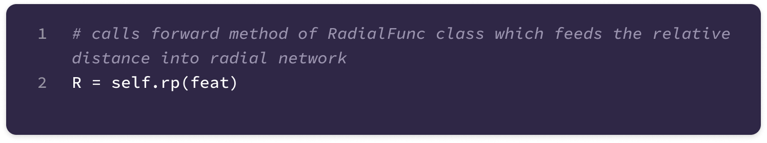
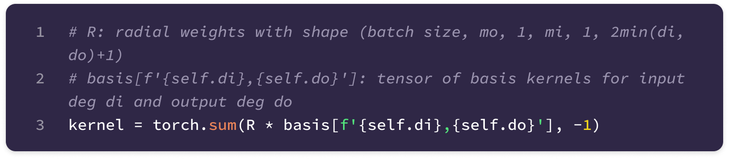
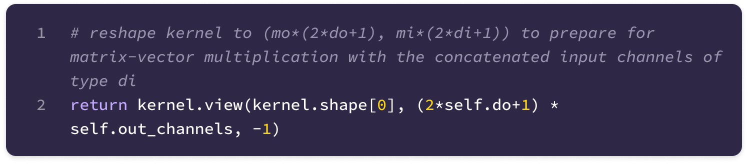
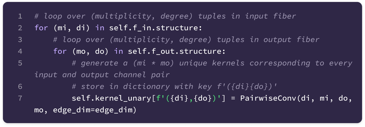
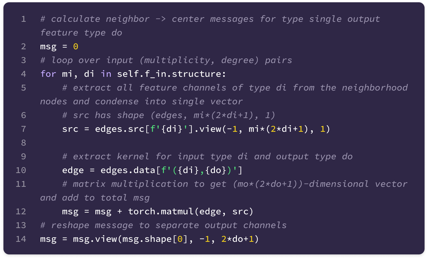
We repeat step 6 for every output feature type and every directional edge in the graph. The neighbor-to-center message for a single output type is stored as an array with shape (edges, mo, 2l+1) and modified with a self-interaction step, which we will break down in the next two sections.
Since each of the n edges (from every neighborhood node) pointing to the center node i generates a mo x (2l+1) type-l message, we need to apply a permutation-invariant reduction operation to reduce the messages across edges into a single output type-l tensor. We achieve this by taking the mean across the type-l messages from all n incoming edges which becomes the final type-l neighbor-to-center message to node i.
Now, let’s break down the two types of self-interaction that can be applied to the neighbor-to-center message before aggregation: linear self-interaction and channel-mixing. At the end of the TFN section, we will put all the components together in a user-defined function and see how to generate an updated graph representation with the output messages.
Linear Self-Interaction
The output of the TFN layer also contains a linear self-interaction term added to the message-passing term that incorporates the features from the node itself and acts as an equivariant skip connection or residual connection.
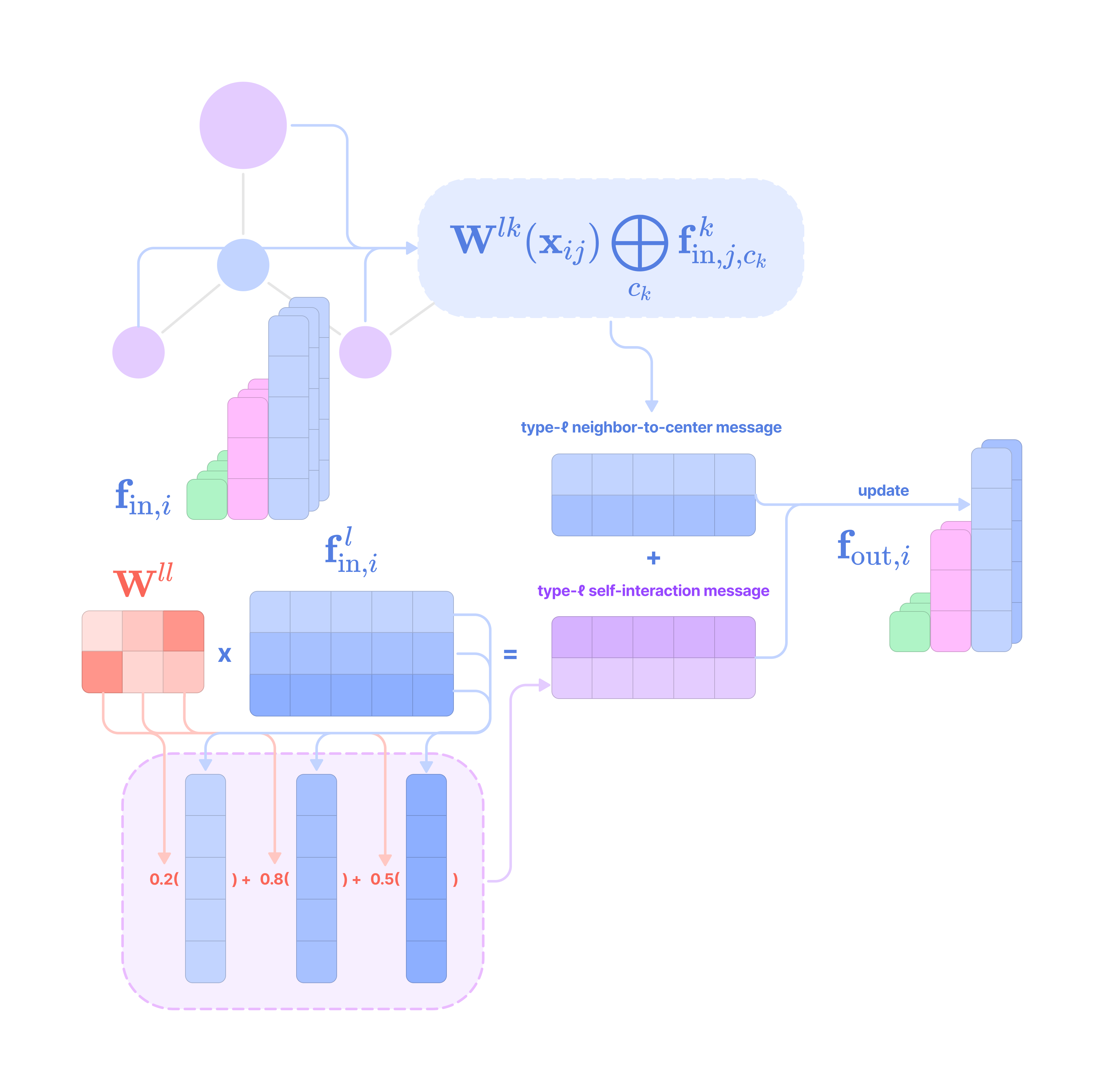
Skip connections in deep learning are a technique used to prevent vanishing gradients by adding or concatenating input data to the transformed output data between layers, which allows the gradient to skip past gradient-diminishing layer operations during backpropagation. In the TFN module, linear self-interaction introduces a skip connection by adding linear combinations of a node’s input features into the output feature tensor. Since the neighbor-to-center message is dominated by features from adjacent nodes, this step also prevents the independent properties of each node from being lost after each feature update.
We cannot transform between different feature types in a single node without a displacement vector, and directly combining different types breaks equivariance. To preserve equivariance, linear self-interaction takes the learnable weighted sum of input channels with the same degree and adds it to the output neighbor-to-center message of that degree.
This expression calculates a type-l self-interaction spherical tensor for the type-l output channel c_l of node i by taking the weighted sum of all the type-l input channels (denoted by c_l’) using a set of learnable weights.
Each unique weight is denoted by a subscript (c_l, c_l’) that indicates the input channel c_l’ that is being scaled by the weight and the output channel c_l for which the self-interaction is being calculated, and this weight is used across every node in the graph.
The self-interaction weights for all type-l channels are stored in a matrix with dimensions (output type-l channels, mo) x (input type-l channels, mi), where each row corresponds to all the weights used to calculate self-interaction for a single output channel.
Let’s break down the implementation for self-interaction:
For each output feature type, a weight array of shape (1, mo, mi) is initialized with random integers and scaled down by the square root of the number of input channels to reduce the variance of outputs.
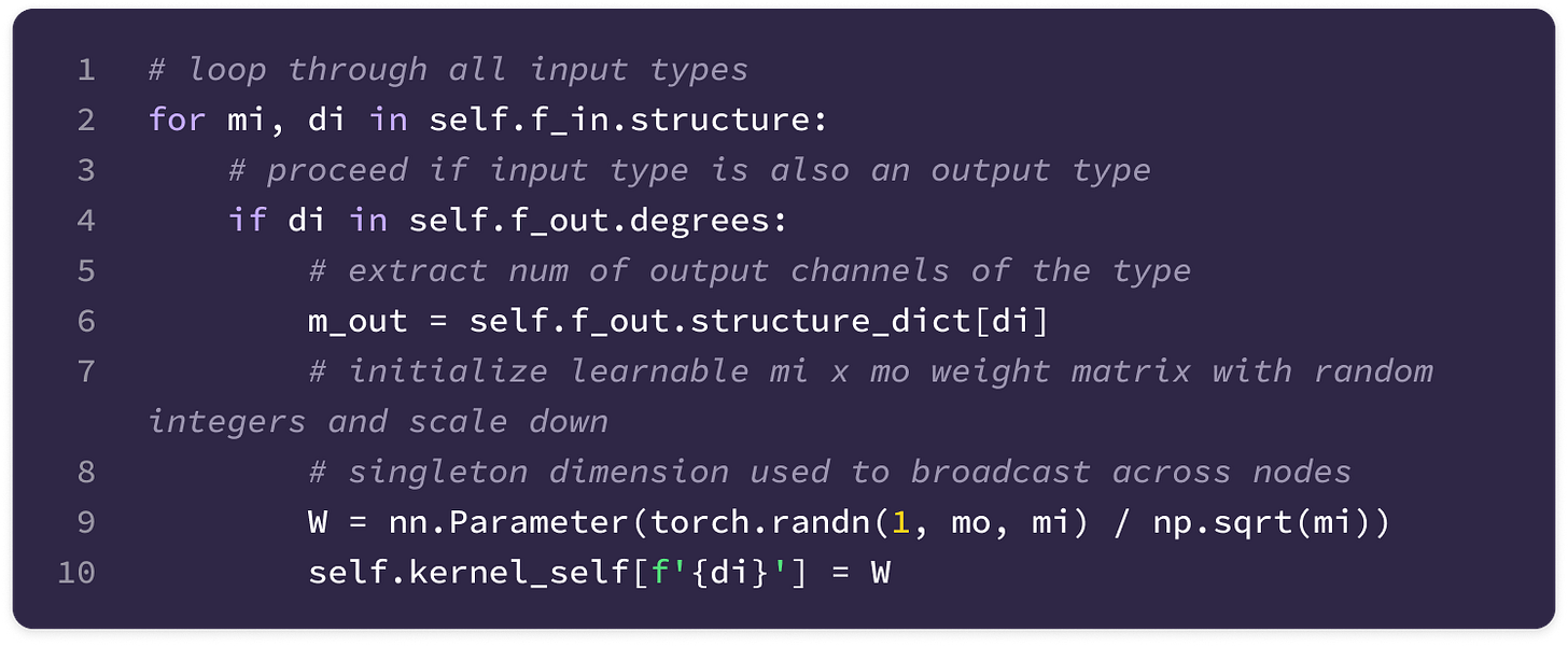
Then, we generate the self-interaction tensor for all type-l output features at node i by multiplying the weight array with the matrix formed by stacking each type-l input feature as rows.
\(\mathbf{W}^{ll}\mathbf{f}^l_{\text{in},i}\)This operation condenses the process of calculating the weighted sum for each type-l channel into a single matrix multiplication step that calculates self-interaction for all type-l channels simultaneously.
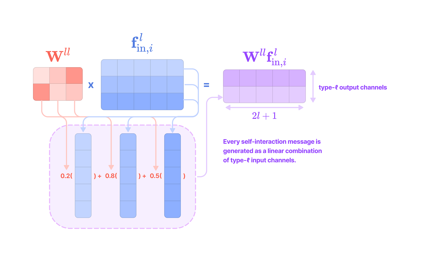
Applying the linear self-interaction weight matrix to the matrix of all type-l input channels stacked into the rows outputs the matrix of self-interaction messages for all type-l output channels. Each row of the output matrix is equivalent to taking the sum of all the input channels scaled by the weights in the corresponding row of the weight matrix. (Source: Alchemy Bio) In the code implementation, this step is performed for every node in parallel by multiplying the weight array with shape (1, mo, mi) with the type-l input feature array with shape (nodes, mi, 2l+1). Based on broadcasting rules, this will produce a tensor with shape (nodes, mo, 2l+1).
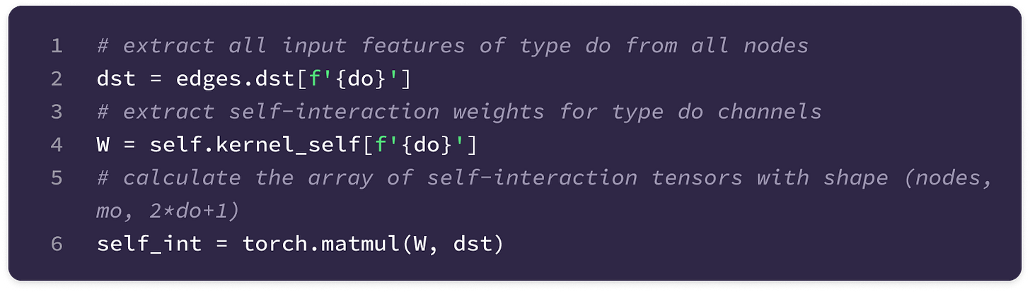
Lastly, the self-interaction array is added to the neighbor-to-center message with the same shape (nodes, mo, 2l+1) for every output degree.
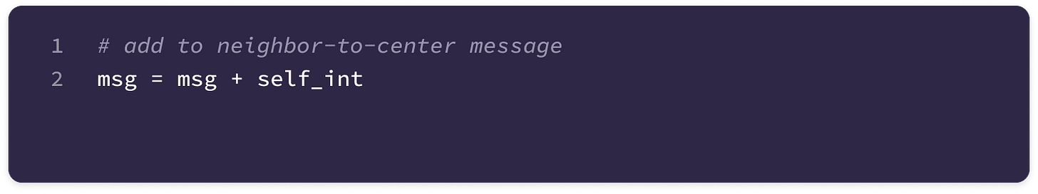
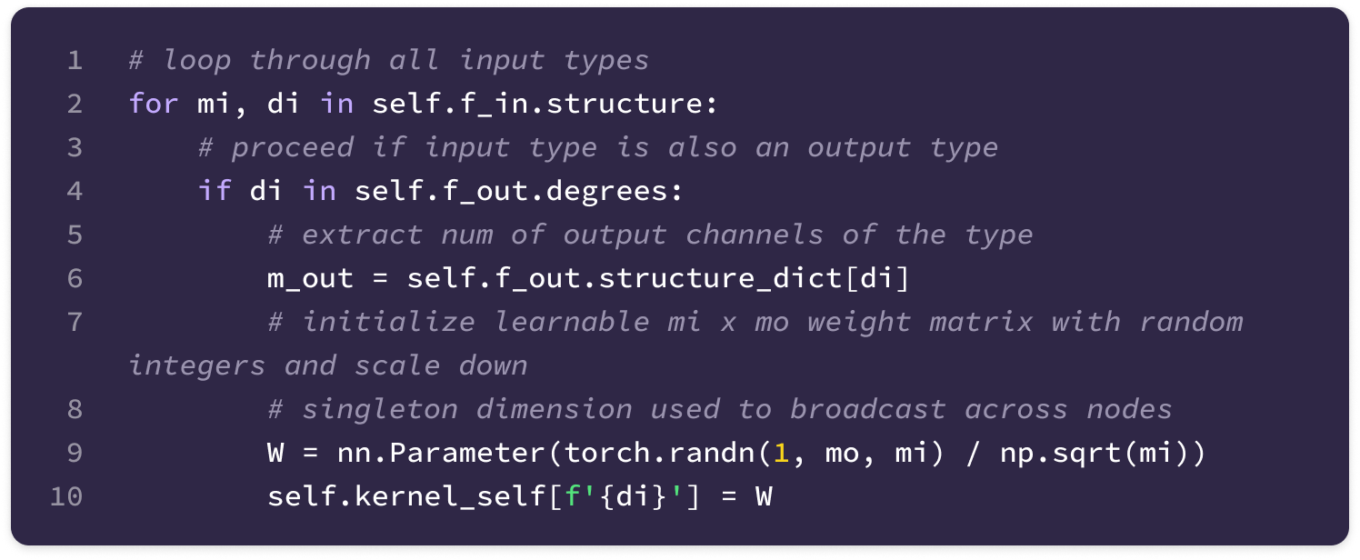

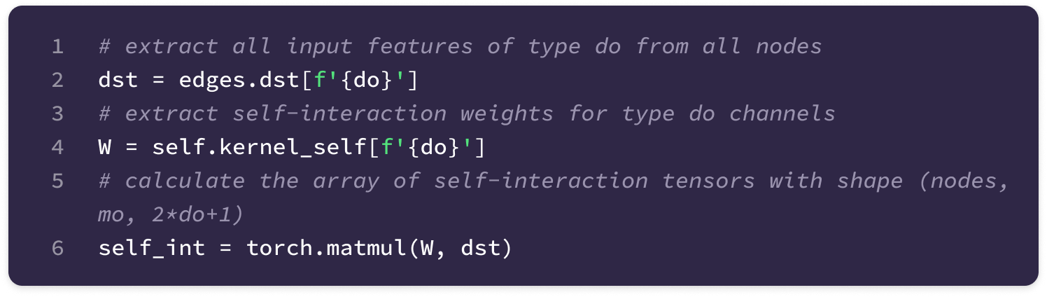
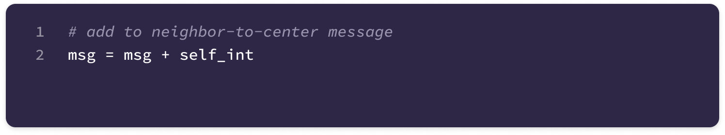
Since the same linear self-interaction message is added to the neighbor-to-center message from every incoming edge to the center node i, we can write the full TFN layer with the equation below:
We will also revisit the linear self-interaction mechanism later when we discuss how to generate the query embeddings for self-attention.
Channel Mixing
Another way to incorporate equivariant self-interaction in a TFN layer is through channel mixing. Since a unique neighbor-to-center message is generated for every channel of every type, instead of simply updating each channel with its corresponding message, channel mixing updates each channel with the weighted sum of the neighbor-to-center messages for all other type-l output channels of the same type.
where the output feature for channel c_l’ inside the summation refers to the neighbor-to-center message before applying channel mixing.
For every output type, there is a corresponding square matrix of learnable weights with dimensions mo x mo, where each row corresponds to the weights used to perform channel mixing for updates to a single output channel c_l.
Instead of multiplying by the input type-l channels like in linear self-interaction, channel-mixing is implemented by multiplying the weight matrix with the matrix formed by the output type-l channels as rows, which outputs a matrix of type-l output messages from node j where each channel is a ‘mix’ of the other channels.
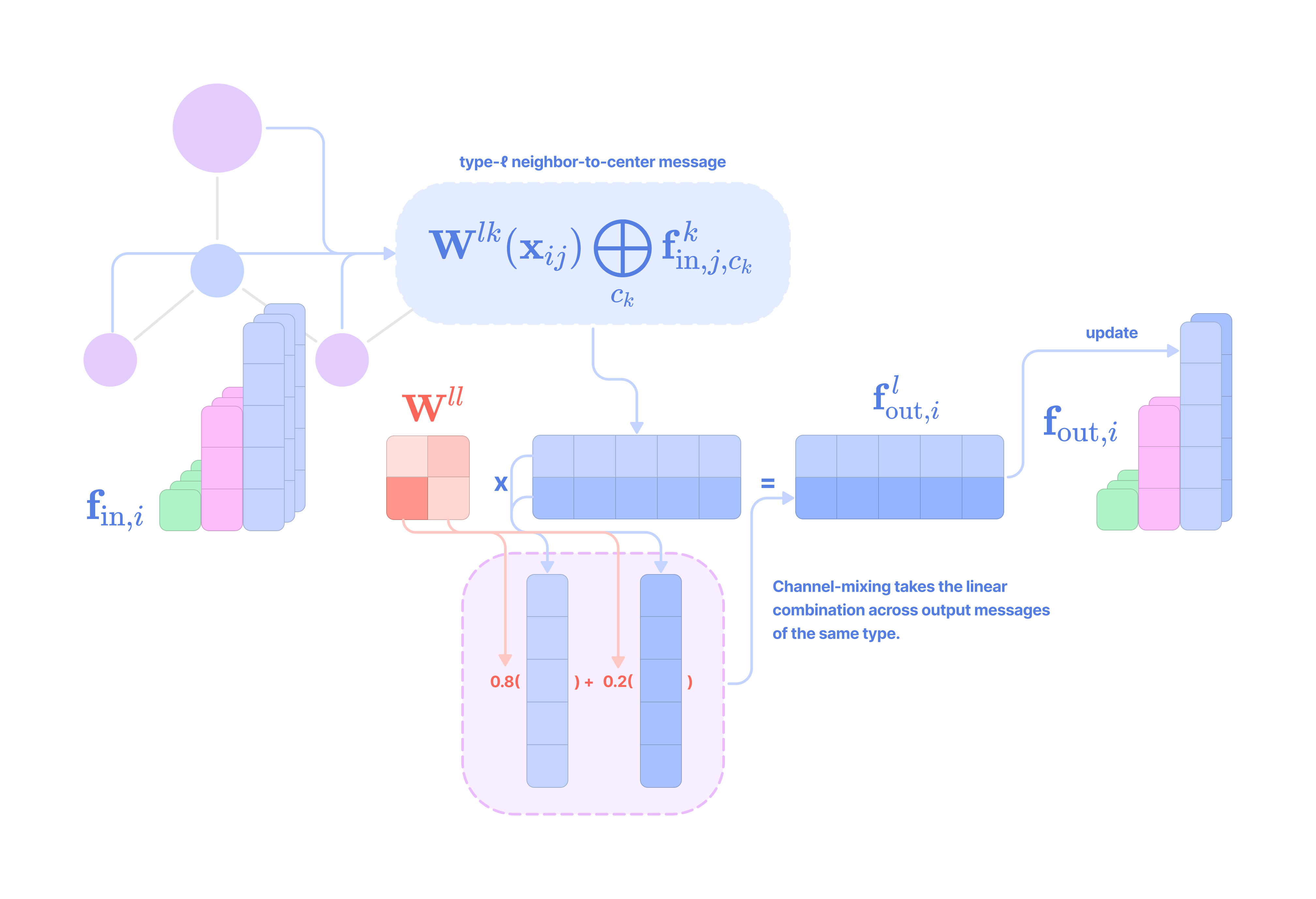
In the code implementation, the weight array of shape (1, mo, mo) is broadcasted and multiplied by the array of all output type-l tensors generated in the message-passing step of shape (nodes, mo, 2l+1) to produce the mixed type-l output message with the same shape.
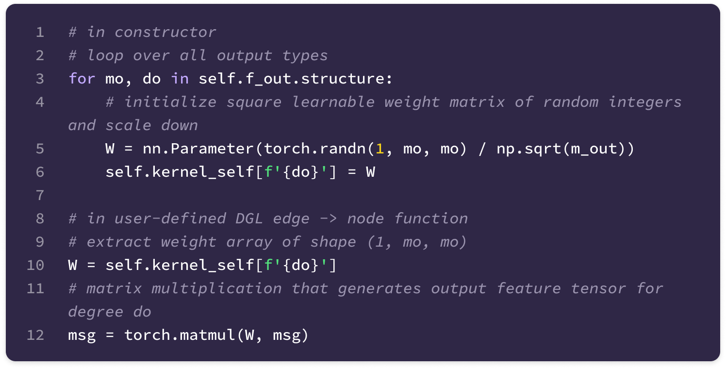
To encapsulate the code for the neighbor-to-center message and self-interaction message, we define an edge UDF in DGL called udf_u_mul_e that computes the messages for a single output feature type for each edge with either linear self-interaction or channel mixing. The messages are stored in a dictionary where the label ‘msg’ is linked to an array with shape (edges, type-l output channels, 2l+1).
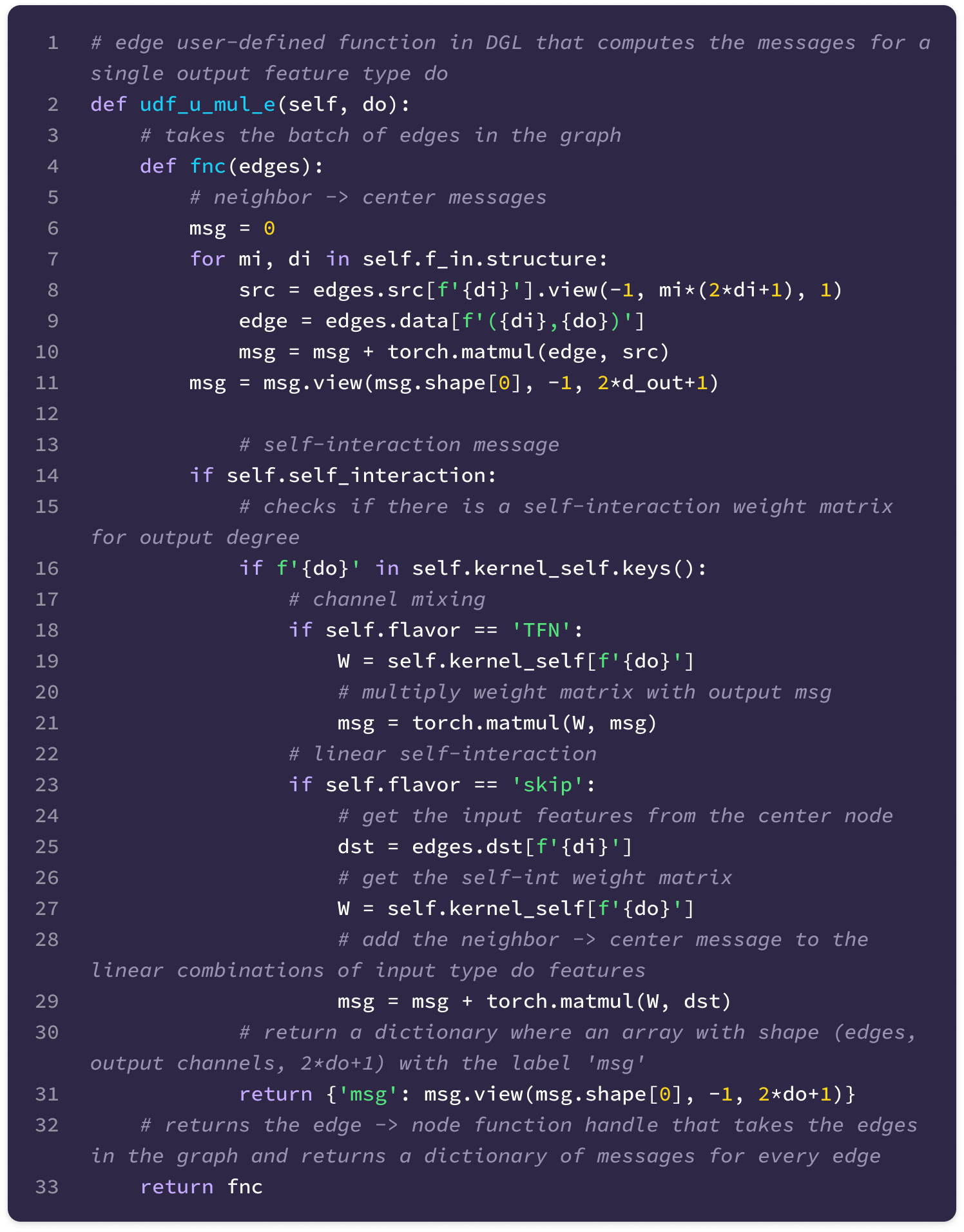
Then, we can loop through every output degree type and call the built-in update_all function in DGL which executes the udf_u_mul_e function and reduces the output messages using the built-in mean function that extracts the array labeled ‘msg’ generated from the udf_u_mul_e function, takes the average of the messages of a given type across all edges that share a destination node, and stores them in the node features of the graph with the label f`out{do}.`
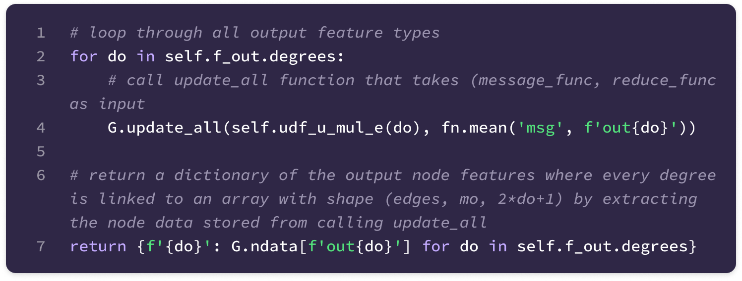
Passing the graph through the full TFN module generates a fully updated graph representation that integrates neighbor-to-center and self-interaction messages.
Now that we understand how equivariant message passing is performed in a tensor field network, we can extend the core mechanisms to construct the SE(3)-Transformer module that incorporates the attention mechanism.
SE(3)-Transformer Module
The Transformer model introduced in 2017 by Vaswani et al. uses the attention mechanism to learn dependencies between distant tokens in sequence data. The SE(3)-Transformer by Fuchs et al. leverages the attention mechanism to weight certain messages between nodes with greater importance than others with scalar attention scores. Attention scores are calculated from node-based query embeddings generated via linear self-interaction and edge-based key embeddings generated via the message-passing mechanism of TFNs. Instead of aggregating messages uniformly, attention scores introduce an added degree of learnable angular dependence and nonlinearity that increases model performance.
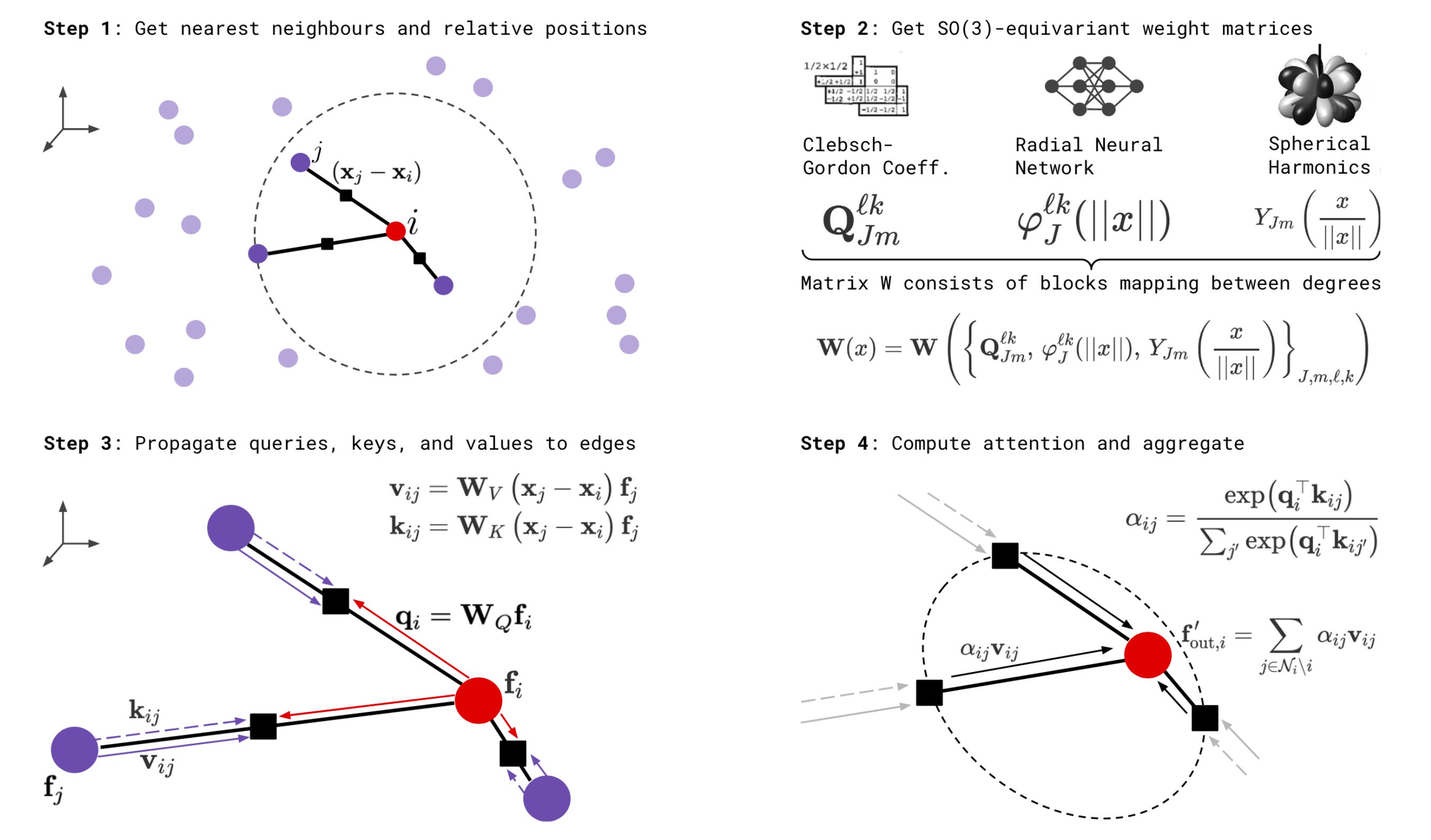
Primer on Self-Attention for Sequences
Before diving into how to assemble an equivariant self-attention layer for geometric graphs, let’s refresh how self-attention is applied to sequence data (e.g. amino acid sequence, small molecule drug SMILES string).
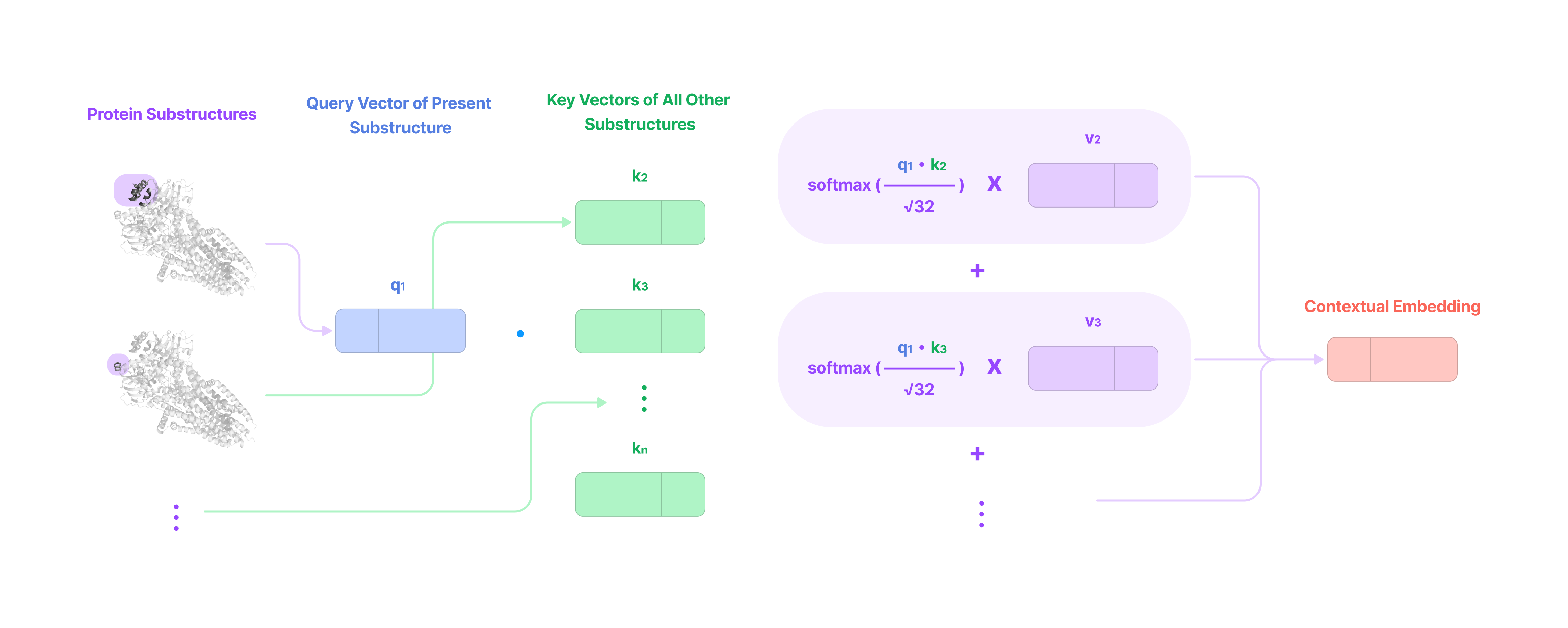
First, the initial embedding of each element in the sequence—containing information on its independent properties and positional information—is converted into a query, key, and value embedding via matrix-vector multiplication with a learnable query, key, and value weight matrix. The dimension of the embedding is generally reduced to facilitate efficient multi-head attention.
To calculate attention on a given element i in the sequence, we take the dot product of the query vector of i with the key vectors of all the other elements in the sequence j ≠ i and normalize with the softmax function to generate a score between 0 and 1 corresponding to each j such that the sum across all elements in the sequence is equal to 1. Higher scores represent stronger relationships (or higher degree of dependency) between the element i with the element j in the representation subspace defined by the set of query, key, and value matrices.
Then, the value vectors for all the elements in the sequence j ≠ i are scaled by their corresponding score and added to generate a learned internal representation or contextual embedding of the element i. This contextual embedding not only holds information on the element itself but also describes its relationship with every other element in the sequence.
Multi-head attention generates multiple attention scores by multiplying the initial embedding with multiple sets of learned query, key, and value matrices, each of which projects the embeddings to a new representation subspace that captures a particular type of relationship between elements in the sequence.
The contextual embeddings from each attention head are concatenated and multiplied with an additional learned weight matrix that captures the relative importance of each representation subspace in describing the element, aggregating all the representations into a single embedding.
Finally, the contextual embeddings for all elements in the sequence are passed into a conventional neural network that generates a prediction for a classification or regression task.
See my previous article on Transformers for Drug-Target Interaction (DTI) Prediction for a deeper look into how self-attention can be applied to small molecule drugs and protein sequences.
Self-Attention for Geometric Graphs
Due to the equivariance constraint, there are no learnable parameters with angular dependence in the TFN module. The kernel generated from the angular unit vector has fixed angular dependence and cannot incorporate dynamic learnable parameters without breaking equivariance, limiting the ability of the kernels to learn complex angular dependencies between nodes.
The SE(3)-Transformer overcomes this challenge by incorporating SE(3)-invariant attention scores computed from query and key embeddings dependent on both learnable parameters and fixed angular basis kernels. These scores are then used to scale the value embeddings for each edge, adding an extra degree of freedom for capturing angular relationships between nodes.

The equation below describes the full mechanism of the SE(3)-Transformer module:
In summary, self-attention can be applied to generate a message for a node i with the following steps:
The features at each node are transformed into a node-based query embedding by applying linear self-interaction across same-degree channels with a set of learnable weight matrices, generating each output query tensor channel as a linear combination of all input channels of the same type. The query tensors for every channel of every degree are concatenated into a single query embedding associated with the center node.
An edge-based key embedding with the same dimension as the query embedding is generated for every directional edge in the graph in the same way as the neighbor-to-center messages of the TFN layer.
The dot product between the query embedding of the center node and the key embedding for each incoming edge computes the raw attention scores associated with each incoming edge.
The raw attention scores across edges that share the same destination node are fed into the softmax function, which normalizes the scores into a set of probabilities that sum to 1.
Instead of taking the average message over all incoming edges to the center node like the TFN module, the SE(3)-Transformer scales a value message generated for each edge by the associated attention score and takes the sum to get the aggregated neighbor-to-center message.
Then, the input features from the center node are concatenated to the neighbor-to-center and fed into an attentive self-interaction layer, which projects the concatenated tensor to match the output fiber. A matrix of weights is uniquely computed for each node with the attention mechanism and multiplied by the concatenated tensor to generate the final output message.
Now, let’s break down the implementation of these steps in detail.
Computing the Query Embedding
The query embedding serves as a representation of the center node that is used to look up specific interactions and motifs in the features of neighboring nodes that are relevant in updating its position and feature tensors. In the context of modeling proteins, the query embedding could contain data relevant to determining an amino acid’s interaction with other amino acids such as hydrophobicity, charge, and the torsion angles between N-Cα and Cα-C bonds.
The query embedding is a node-based embedding, which means it should only be dependent on the features of the node itself because it will be used to calculate the attention weights for all incoming edges.
Since we cannot transform between different feature types in a single node without the displacement vector, we use the linear self-interaction mechanism described earlier to project each input feature type to their specified number of output channels, where each output channel is the learnable weighted sum of all input channels of the same type.
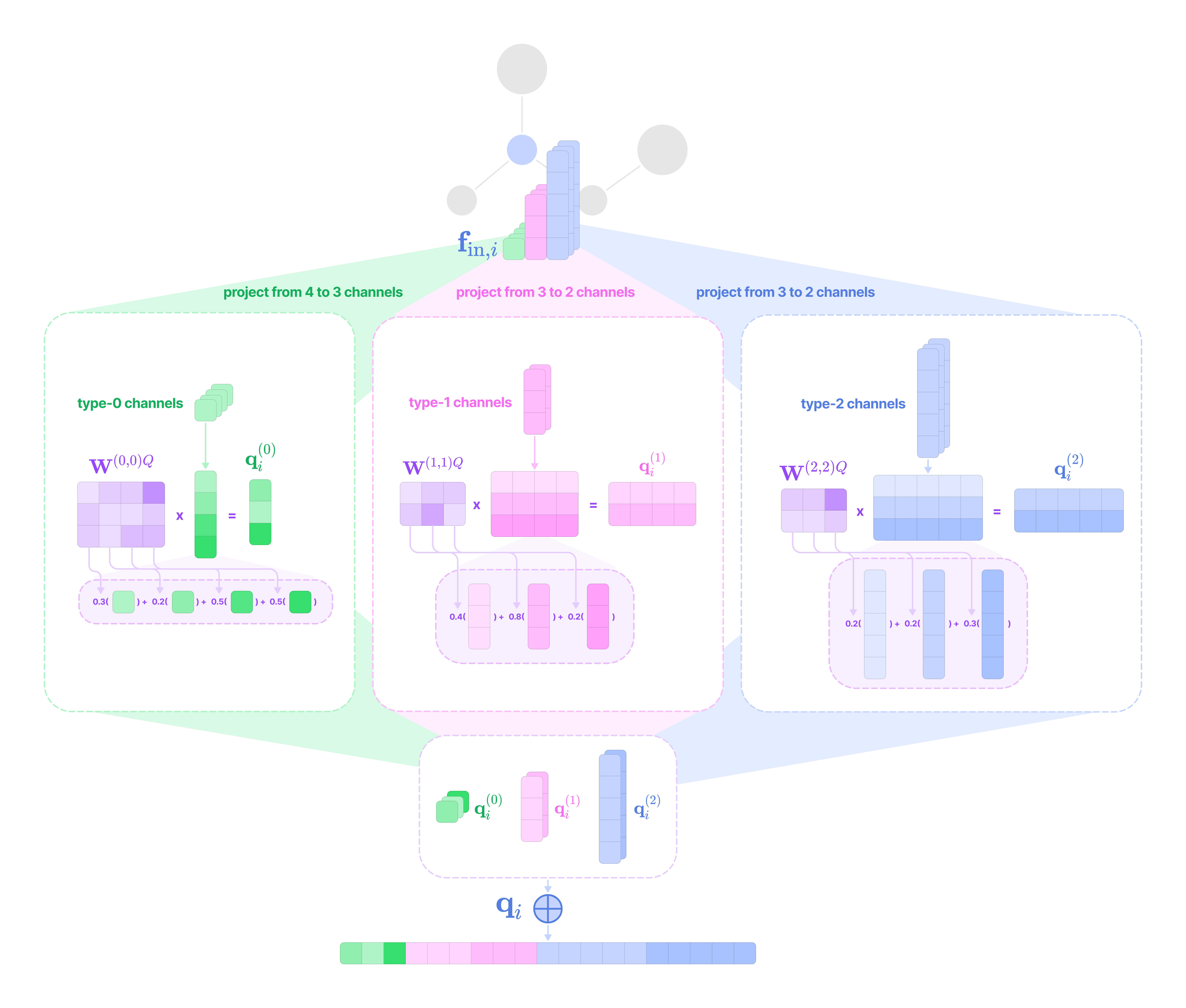
To determine the dimensions of the query embedding, we can define a new fiber structure called f_mid_in that contains (multiplicity, degree) tuples corresponding only to degrees in both the input and output fiber but with the same number of channels as the value messages of the self-attention layer.
To illustrate, if the input fiber to the attention layer has structure [(4, 0)] and the value fiber f_mid_out has structure [(16, 0), (16, 1), (16, 2), (16, 3)], f_mid_in has structure [(16, 0)], meaning the full query embedding will consist of 16 channels of type-0 tensors.
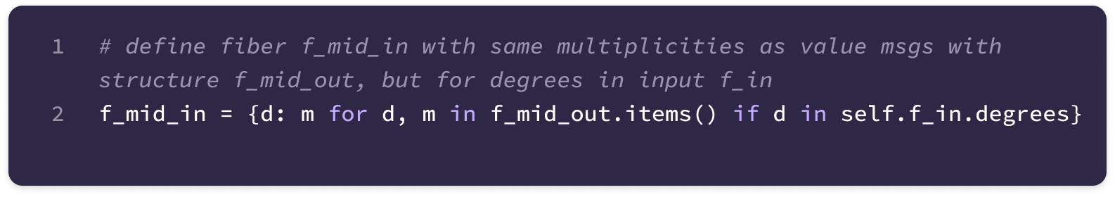
Now that we have defined its structure, let’s break down how to calculate the query embedding for the center node i:
The learnable weights are stored for each input degree as a query weight matrix with the following dimensions:
\(\mathbf{W}^{llQ}\in \mathbb{R}^{(\text{type-}l\text{ channels in value message})\times \text{(type-}l\text{ input channels})}\)We define a dictionary of weight matrices where each degree l is linked to a query weight matrix. The weights are initialized with random integers that will be optimized with gradient descent and scaled down by the number of type-l input channels, mi:
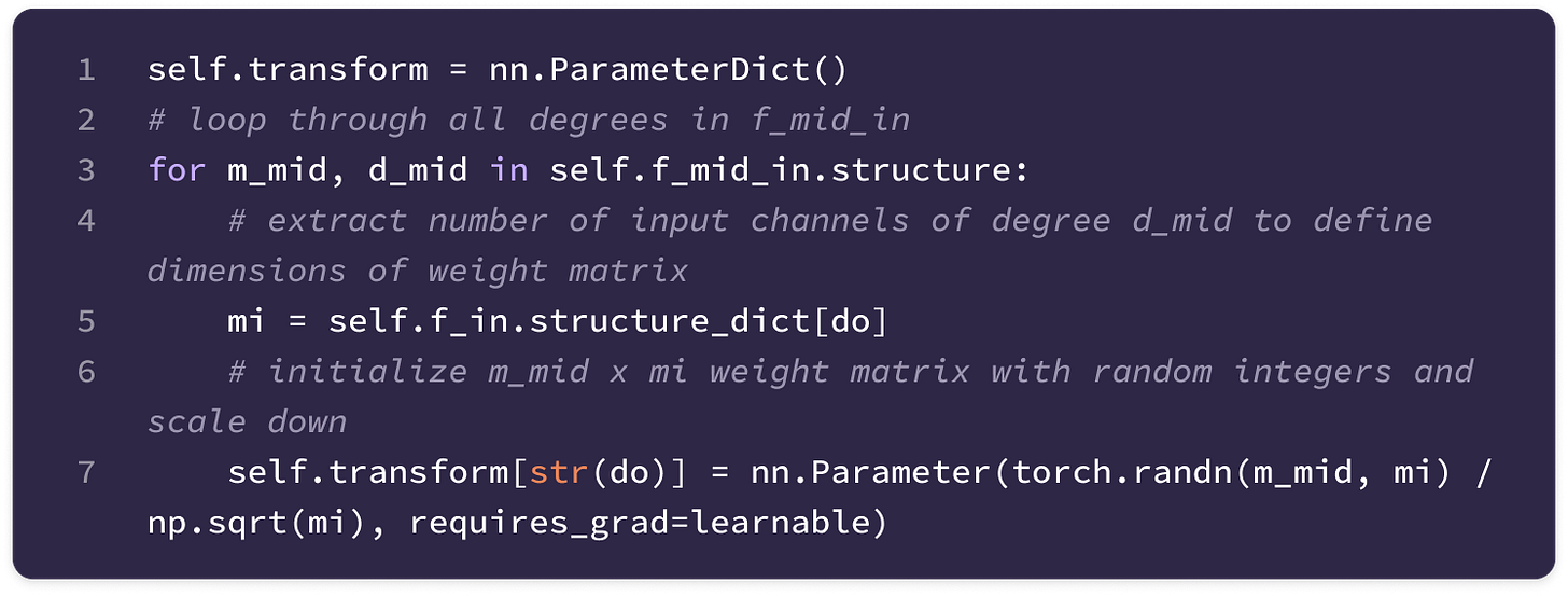
The query embedding for a single type-l output channel c_l is generated as a weighted sum of all type-l input channels (indexed by c_l’) using the weights in the c_lth column of the query matrix:
\(\mathbf{q}^l_{i,c_l}=\sum_{c_l'}w^{ll}_{c_l',c_l}\mathbf{f}^l_{\text{in},i,c_l'}\)We can compute query embeddings for every type-l output channel simultaneously by multiplying the query matrix with all the type-l features stacked horizontally into a (input channels) x (2l+1) matrix, producing an (output channels) x (2l+1) matrix where each row is the query embedding for a single output channel. This operation is equivalent to separately computing the weighted sum for every type-l output channel using the equation from step 2 and stacking the outputs into the rows of a matrix.
\(\mathbf{q}^l_{i}=\text{vec}(\mathbf{W}^{llQ}\mathbf{f}^l_{\text{in},i})\)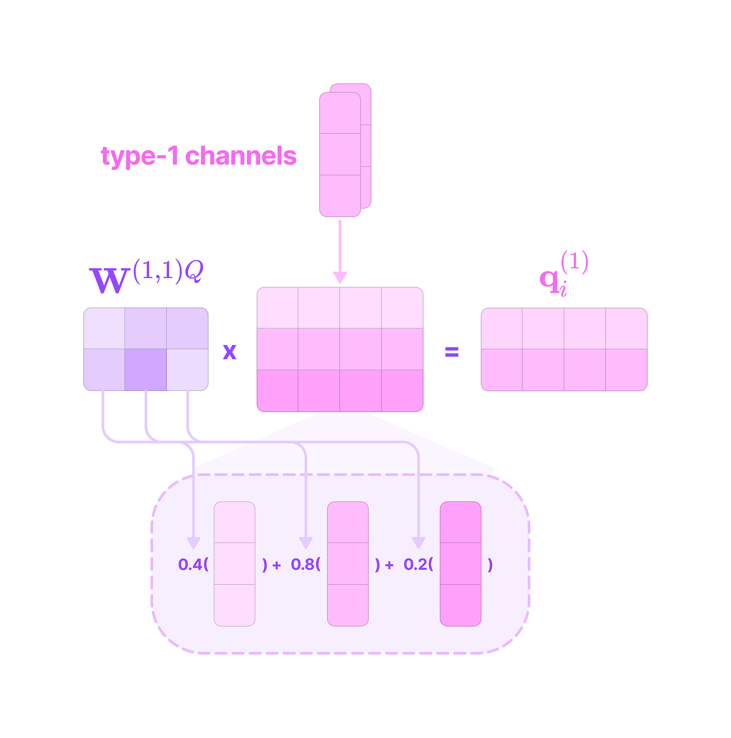
The type-1 query embedding is generated as the weighted sum of the type-1 input features. The 3 type-1 input channels are transformed into 2 type-1 output channels by multiplying by the query weight matrix with superscript (1,1) indicating it is transforming between type-1 and type-1 tensors. (Source: Alchemy Bio) With the query matrices, we can implement the code that generates the matrix of type-l output query embeddings for every node in the graph:
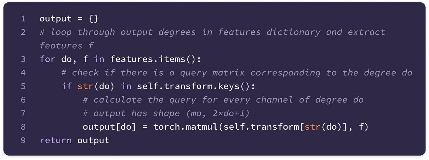
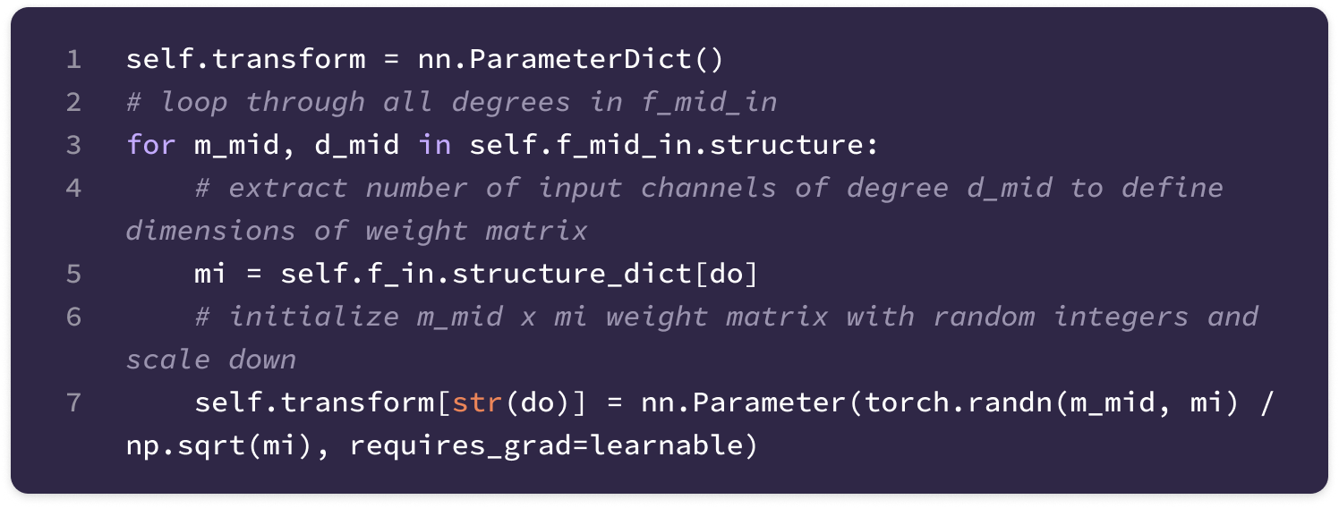

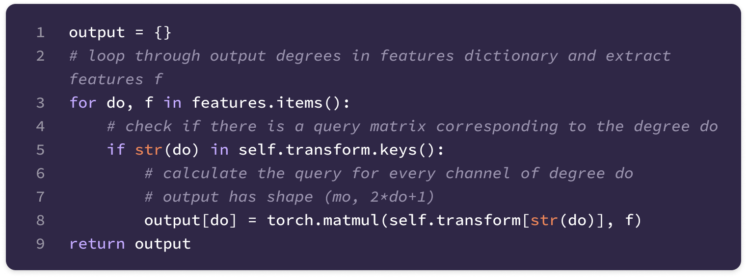
Finally, we repeat this step for every degree defined in f_mid_in. The code above is implemented in the G1x1SE3 module for linear self-interaction that is called in the GSE3Res module to generate a list of query arrays for every node in the graph, where the lth element of each list is an array of type-l queries with shape (type-l channels in f_mid_in, 2l+1):
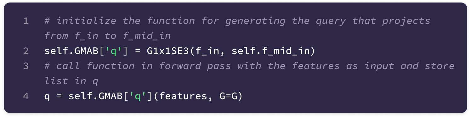
Before we calculate the attention scores, we have to reshape the query embedding into a single vector that can be used to take the dot product with the key embeddings. We do this by (1) concatenating the queries across all channels of each degree by squeezing the last two dimensions corresponding to the channel and tensor-component axis of each array into a single dimension and (2) concatenating the embeddings of all degrees by squeezing along the last dimension of the array. This is implemented with the following helper function with the number of attention heads set to 1 for now:
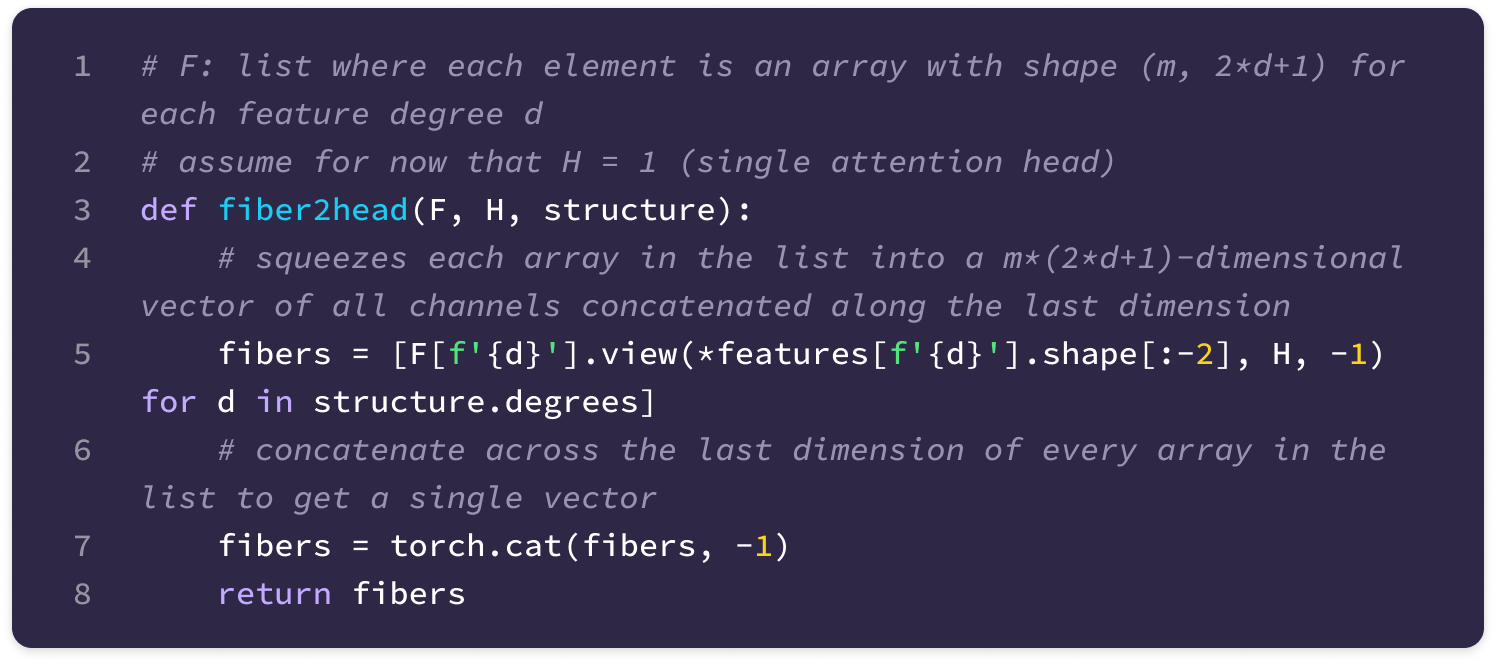
Now, we can call this function to concatenate all the query embeddings for all output type-l channels c_l in the value fiber and all input degrees l to get the full query embedding for node i:
Computing the Key Embeddings
While the query embedding serves as a lookup tool that searches for relavent interactions and features from neighboring nodes, the key embedding serves as the dictionary of all interactions and feature motifs from neighborhood nodes that the query of the center node is compared to. If the query and key for a given edge are similar (large dot product), more weight is placed on the value message generated from that edge.
The key embedding is an edge-based embedding generated in the same way as the neighbor-to-center message in the TFN module without self-interaction. For each edge, the key embedding is generated by transforming every feature in the source node with uniquely defined equivariant kernels constructed with learnable radial weights and spherical harmonics with angular dependence, such that the embedding contains information on both the source node and the edge features between the source and center node.
Note that the key embeddings for the edge from node j to i and the edge from node i to j are different, so each node has a unique set of key embeddings corresponding to every incoming edge from nodes in the neighborhood centered around it.
Since the dimension key embedding must align with the query embedding to compute the element-wise dot product, we use the f_mid_in fiber as the output fiber of the neighbor-to-center message computation to ensure that the multiplicity for each type of key embedding aligns with the query. From now on, we will refer to the multiplicity for an arbitrary but particular degree l in f_mid_in as mid.
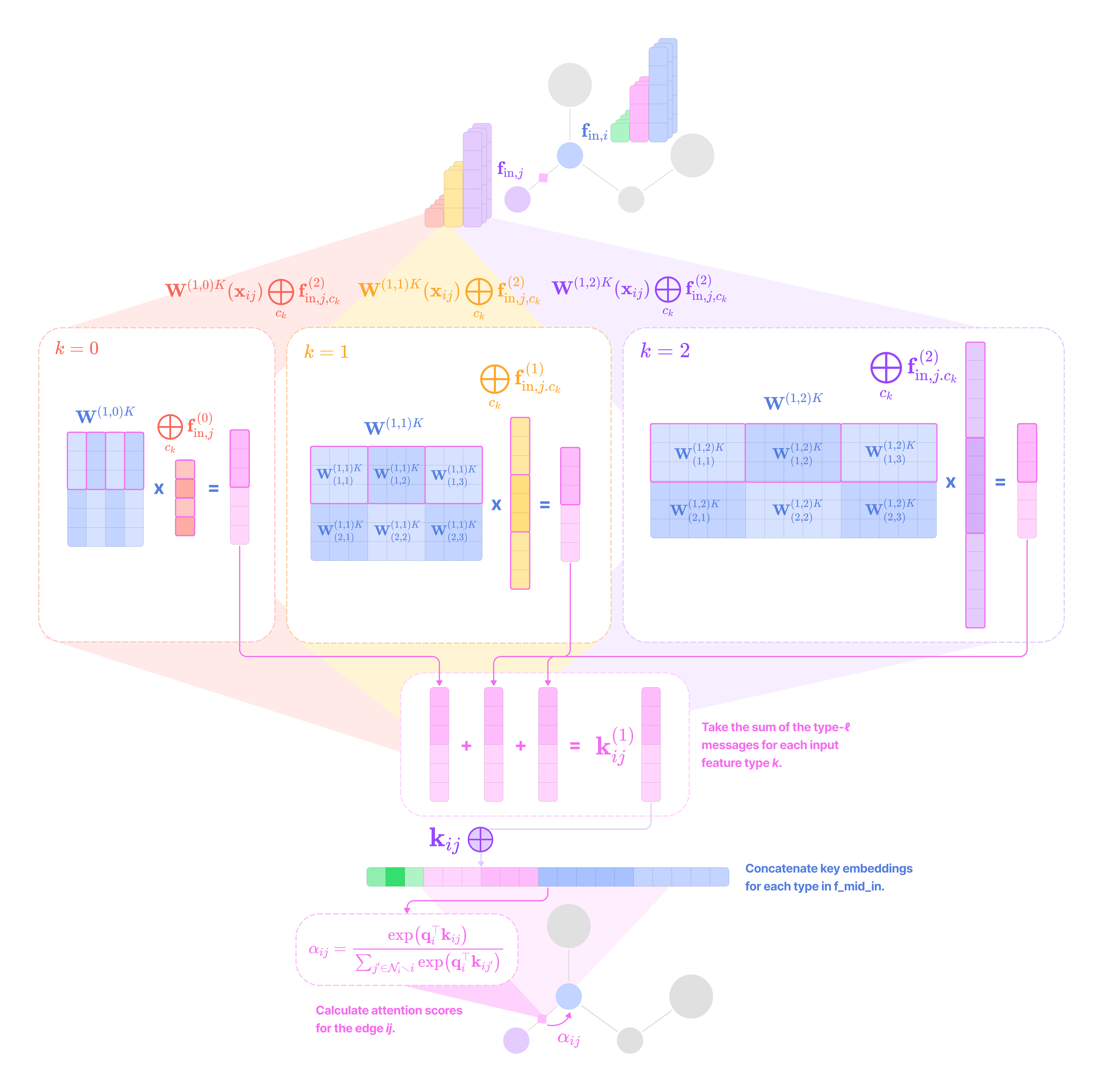
Let’s break down how to generate the type-l key embedding for the edge from node j to node i:
For computing all key embeddings across every edge, a set of key radial functions (denoted by the superscript K) are defined for every ordered pair of input and output degrees (k, l), each of which outputs a (mid)*(type-k input channels, mi)*(2min(l,k)+1)-dimensional vector of weights for every input radial distance.
\(\varphi^{lkK}(||\mathbf{x}_{ij}||):\mathbb{R}^3\to \mathbb{R}^{{\text{(mi)*(mid)*}(2min(l,k)+1)}}\)From the key radial function, we construct a (mid)*(2l+1) x (mi)*(2k+1) equivariant key kernel that transforms all the type-k input channels from node j to the number of type-l output key embeddings defined in f_mid_in.
\(\mathbf{W}^{lkK}(\mathbf{x}_{ij})=\begin{bmatrix}\mathbf{W}^{lkK}_{(1,1)}&\mathbf{W}^{lkK}_{(1,2)}&\dots&\mathbf{W}^{lkK}_{(1,\text{mi})}\\\\\mathbf{W}^{lkK}_{(2,1)}&\ddots&\dots &\vdots \\\\\vdots &\dots &\ddots& \vdots\\\\\mathbf{W}^{lkK}_{(\text{mid},1)}&\dots &\dots &\mathbf{W}^{lk}_{(\text{mid},\text{mi})}\end{bmatrix}_{(\text{mid}*(2l+1))\times(\text{mi}*(2k+1))}\)Each block of the lk key matrix is the (2l+1) x (2k+1) matrix that transforms a single type-k input channel c_k to a single type-l key embedding for channel c_l:
\(\mathbf{W}^{lkK}_{(c_l,c_k)}(\mathbf{x}_{ij})=\sum_{J=|k-l|}^{k+l}\varphi^{lkK}_{(J,c_l,c_k)}\mathbf{W}^{lk}_J(\mathbf{x}_{ij})\)The key weight matrices are generated with the same code implementation as the kernels in the TFN layer described previously.
Next, we can compute a corresponding key embedding for every type-l channel in the query embedding by taking the matrix-vector product between the key kernel defined above and the direct sum of all type-k input channels from node j.
\(\mathbf{k}^l_{ij}=\bigoplus_{c_l}\mathbf{k}^l_{ij,c_l}=\underbrace{\sum_{k\geq0}\underbrace{\mathbf{W}^{lkK}(\mathbf{x}_{ij})\bigoplus_{c_k}\mathbf{f}^k_{\text{in},j,c_k}}_{\text{key emb from type-}k\text{ input channels}}}_{\text{sum over type-}l\text{ key embs for all input types }}\)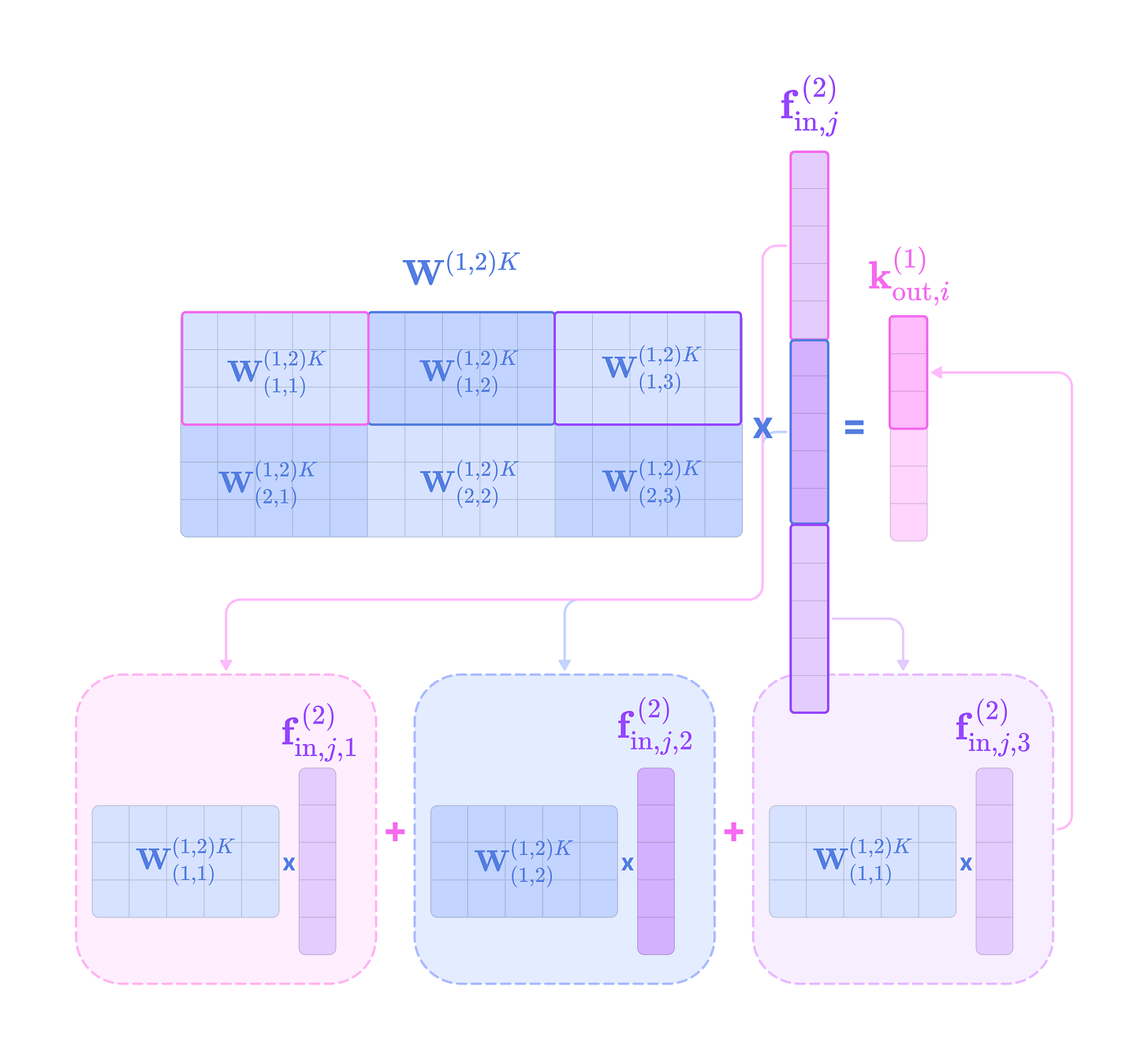
Taking the matrix-vector product between the combined key weight matrix transforming from types k to l and vector concatenation of every type-k input channel is equivalent to separately multiplying a row of (2l+1) x (2k+1) blocks in the key kernel with the corresponding type-k input channel, and taking the sum of the type-l outputs to get a single channel of the type-l key embedding. Each row of kernels in the combined key kernel transforms the type-k input channels into a single type-l output channel. (Source: Alchemy Bio) The code to implement this calculation is the same as step 6 in the section on equivariant message-passing, except with the incorporation of edge features, which we will discuss later.

The keys for every degree in f_mid_in are generated with the same process as step 3, only with a new set of key kernels.
In the code implementation, we loop through all the degrees in f_mid_in and call the udf_u_mul_e UDF defined the same way as the TFN module which computes all the type-l key embeddings for every edge in the graph and stores it in a dictionary with a single label f`out{l}` linked to an array with shape (edges, mid, 2l+1). Then, the dictionary is stored in the edge data by calling the built-in apply_edges function in DGL.
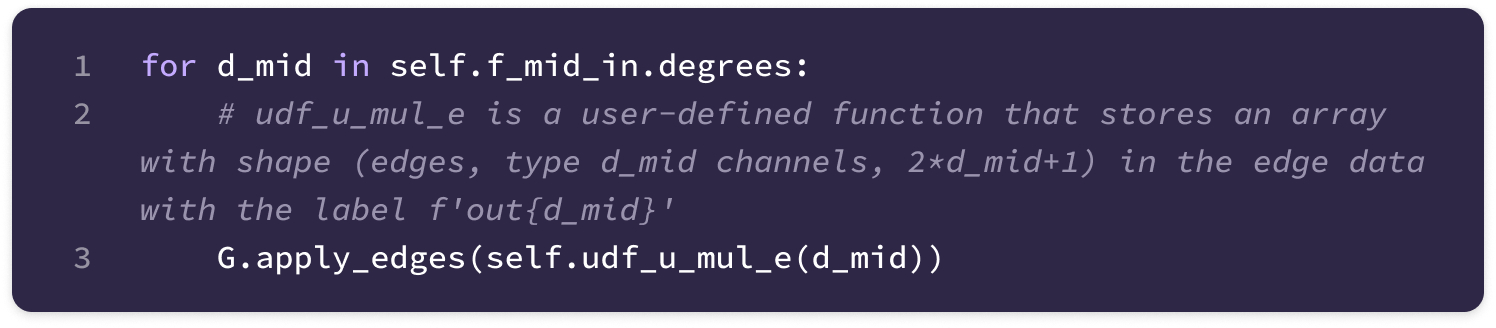
Then, we return a dictionary where every degree is linked to a list of all the key embedding channels of that type for every edge.
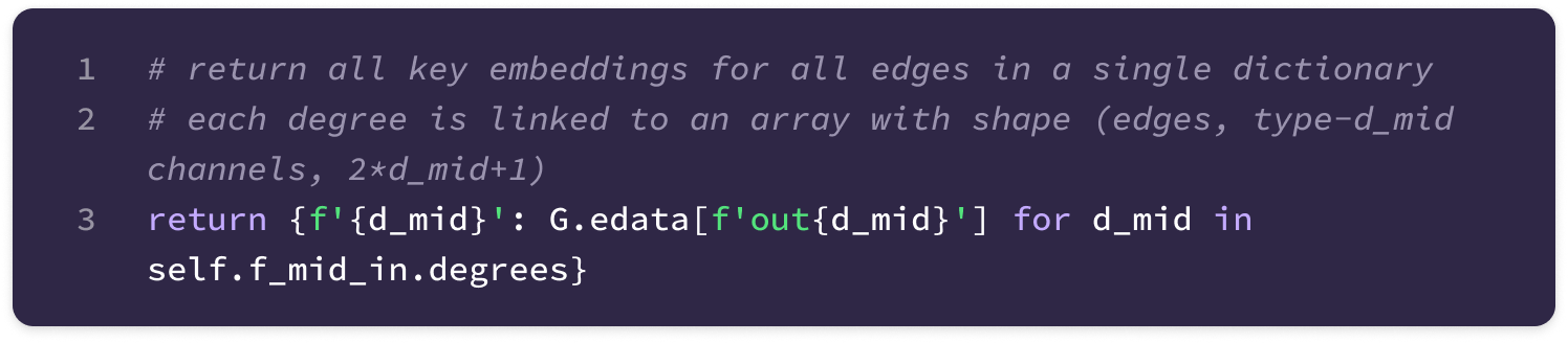
The code above is implemented in the module called GConvSE3Partial which is called in the GSE3Res module:
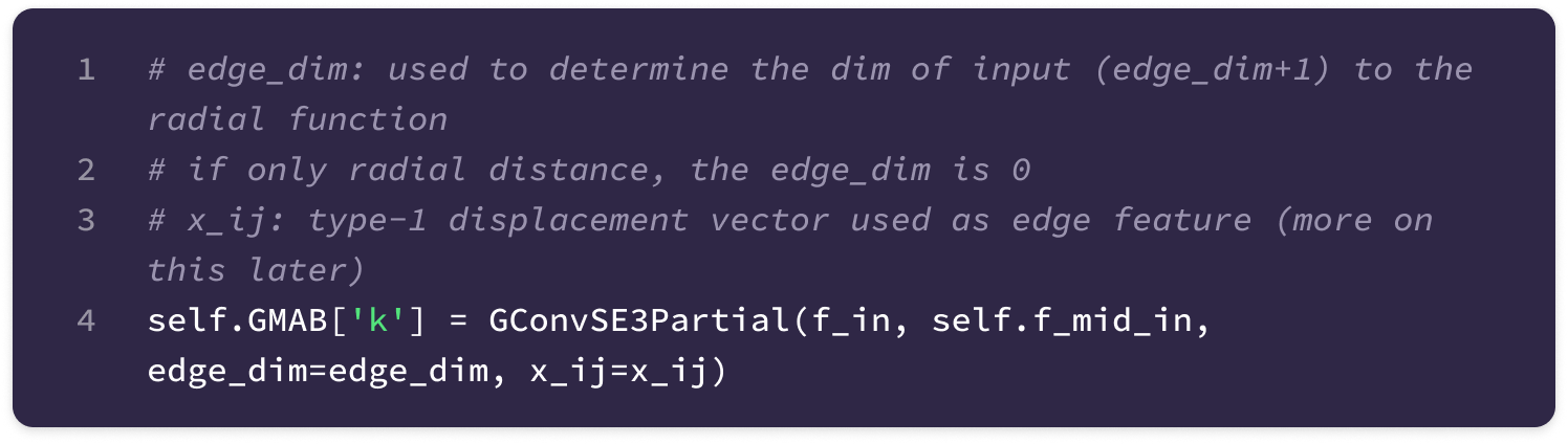
Just like the query embedding, we concatenate the key embeddings for every channel of every type into a single vector with the same dimension as the query embedding for each edge.
This is implemented with the fiber2head function defined earlier:
Now, we have a single key embedding for every edge pointing to node i that forms the complete set of embeddings used to generate the set of attention scores for node i:
Calculating Attention Scores
For each node in the graph, we compute a set of SE(3)-invariant attention scores by taking the dot product between the query embedding of the node with the set of key embeddings associated with each incoming edge.
Since the dot product measures the distance between tensors, the raw attention scores indicate the similarity between the query representation of node i and the key representations of each neighborhood node. The key representations are encoded with learnable parameters, so they are trained to represent features from neighborhood nodes with strong interactions with the center node such that they produce large attention scores with the query embedding while representing features irrelevant to the center node such that they produce low attention scores.
To illustrate, consider a model tasked to predict the interaction between amino acids in a protein. The parameters in the key matrix for a given edge can learn to transform the node features of the ‘source’ residue carrying a positive charge into a key embedding that produces a large dot product with the query embedding of the ‘center’ residue carrying a negative charge.
In single-head attention, a single attention score (denoted by α) is computed for each edge ij and used to scale all channels and feature types in the value message from the source node j. The set of all scores for the center node i can be calculated as follows:
First, we take the dot product between the query embedding of node i and all the key embeddings of incoming edges to generate the set of raw attention scores:
\(\mathbf{q}_i\cdot\mathbf{k}_{ij}=\mathbf{q}_i^{\top}\mathbf{k}_{ij}\)The following code uses the built-in e_dot_v DGL function to calculate the set of raw attention scores for every node in the graph from the set of keys of incoming edges. In other words, e_dot_v computes a scalar value for every edge in the graph that is equal to the dot product between the key of the source node and the query of the destination node of the edge. Since the key array has shape (edges, heads=1, query dimension) and the query has dimension (nodes, heads=1, query dimension), the function first broadcasts the query array such that every key embedding of an edge pointing to the same node is multiplied with the same query embedding. The output of the function is an array with shape (edges, heads=1) that is stored in the edge data labeled ‘e’ by calling the apply_edges function:
Then, we divide each score by the square root of the dimension of the query and key vector d, which equals the sum of (mid)*(2l+1) for all values of l in f_mid_in. This prevents the dot product from growing too large and pushing the gradient to zero after applying the softmax function.
\(\frac{\mathbf{q}_i\cdot\mathbf{k}_{ij}}{\sqrt{d}}\)The dimension d of the key and query fiber is stored in n_features, an instance variable of the fiber object that is calculated by multiplying the number of channels and the dimension of the tensor-component axis for each degree and summing over all degrees in the fiber:
The softmax function is applied separately to each set of raw attention scores of edges that share a center node. This converts the raw scores into a probability between 0 and 1 such that the sum across the set of scores for any given node is 1 (learn more about why the softmax function works here).
\(\alpha_{ij}=\frac{\exp\left(\frac{\mathbf{q}_i\cdot \mathbf{k}_{ij}}{\sqrt{d}}\right)}{\sum_{j'\neq i}^n\exp\left(\frac{\mathbf{q}_i\cdot\mathbf{k}_{ij'}}{\sqrt{d}}\right)}\)This is implemented with the edge_softmax DGL function, which is designed to compute softmax across edges with the same destination node for all edges in the graph.
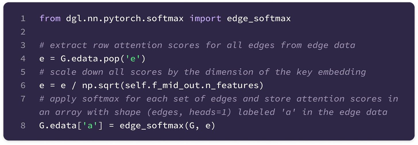
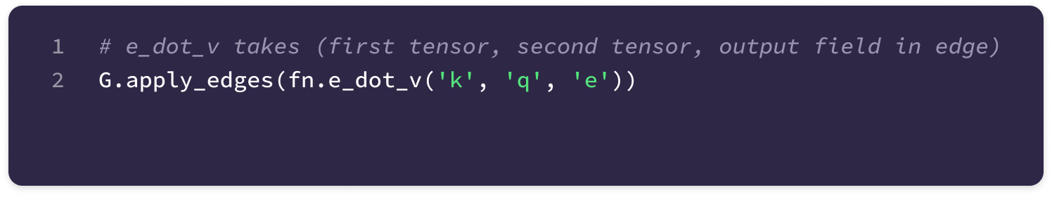
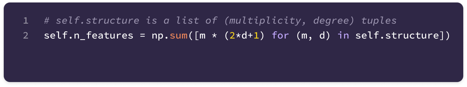
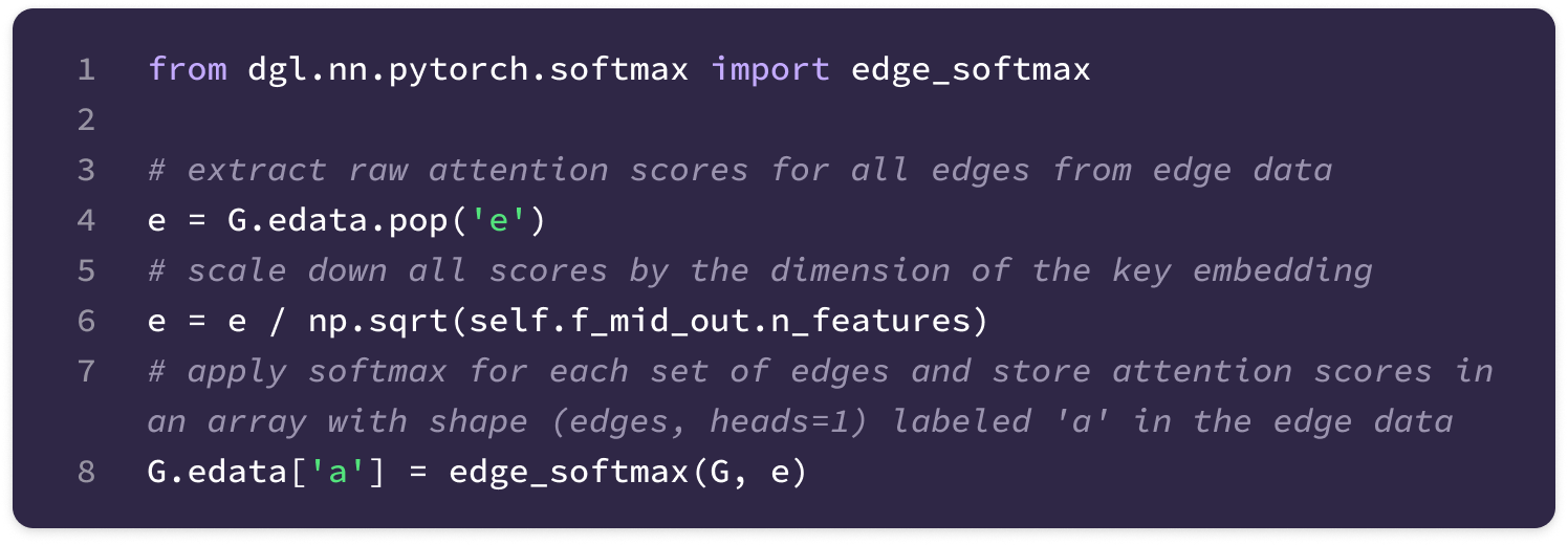
Before moving on, let’s make sure the dot product of the query and key embeddings is SO(3)-equivariant.
We know that each type-l component of the query and key embeddings are SO(3)-equivariant since we constructed the key and query kernels such that they transform under the Kronecker product of type-l and type-k irreps.
Then, we concatenate them into a single embedding in the same order such that the type-l component of the query embedding aligns with the type-l component of the key embedding. This means they both rotate under the same representation formed by the direct sum of irreps (block-diagonal of Wigner-D matrices).
Since representations of SO(3) are orthonormal, meaning they preserve lengths and angles, the dot product (and attention scores) are invariant under rotation:
Computing the Value Messages
The value embeddings for each edge contain the neighbor-to-center messages that will be scaled and added together into a complete message used to update the features at the center node. The contribution made by each value message is determined by their corresponding attention score that indicates whether the source node from which the message is generated has relevant interactions with the center node.
Here, we will break down how to generate the edge-based message, called the value embedding in self-attention, that is scaled by an attention weight and summed together with the weighted value embeddings from all other incoming edges to generate the updated output feature tensor for the center node i.
In the SE(3)-Transformer, the number of channels in the value message is scaled down from the structure of the output fiber. This means that the input feature fiber will be projected to an intermediate fiber structure, called f_mid_out, where the channels for every feature type in the output fiber f_out are scaled down by div before being projected into the total number of channels defined in f_out using attentive self-interaction layer. The intermediate fiber structure is initialized with the following code:
The steps involved in generating the value embedding are exactly the same as the key embedding except instead of projecting the input features to match the structure of f_mid_in, the value embeddings are generated from projecting the input features from the adjacent nodes to match the channels and degrees in f_mid_out by multiplying with a unique set of value kernels generated with a unique set of radial functions. The value kernel that transforms all type-k input channels into the number of type-l value embeddings defined in f_mid_out has the following form :
where mval stands for the multiplicity of degree l in f_mid_out and each block of the lk key matrix is the (2l+1) x (2k+1) matrix that transforms a single type-k input channel c_k to a type-l value embedding for channel c_l:
If the input and output fiber have structure [(0, 32), (1, 32), (2, 32), (3, 32)] and div is set to 2, then f_mid_out has structure [(0, 16), (1, 16), (2, 16), (3, 16)]. When generating the value embeddings, the 32 input channels for a single type k are projected down to 16 type-l value embeddings with a (16*(2l+1)) x (32*(2k+1)) value kernel.
The direct sum of the value embeddings for all type-l channels defined in f_mid_out is calculated by multiplying the combined value kernel with the direct sum of all type-k input channels and summing over the products for all input types just like the type-l key embeddings:
For every output degree, we unvectorize the value embedding into an array with shape (edges, mval, 2l+1). By calling the same udf_u_mul_e UDF and apply_edges function used to compute the keys, we compute the value arrays and store them in the edge data with the label f`out{dval}.`
Then, we return all the value arrays in a single dictionary.
To calculate the output type-l feature tensor for node i, we take the weighted sum of the type-l value messages from all n edges pointing to node i and repeat for every degree in f_out.
In the section on attentive self-interaction, we will project this tensor to match the output fiber structure and incorporate a skip connection. But before we do that, we will first extend the self-attention mechanism to multi-head attention. Since the code implementation is written to generalize to multiple heads, we will also be breaking down the general implementation for single- and multi-head self-attention in the next section.
Multi-Head Self-Attention
In sequence data, multi-head attention computes multiple sets of query, key and value embeddings in parallel to capture distinct representation subspaces that each capture a particular type of relationship between elements in the sequence.
To illustrate the purpose of multi-head attention, consider a node in a graph representing the amino acid cysteine. Cysteine is non-polar, hydrophobic, and has the special property that its thiol group (-SH) reacts with the thiol groups of other cysteine residues to form a disulfide bond (R-S-S-R). Therefore, one feature channel for cysteine could indicate its hydrophobic property, and another could indicate the presence of the thiol group. A single attention head can detect the attractive forces between cysteine and other hydrophobic residues by generating a query embedding of the cysteine residue that looks for key embeddings with motifs that indicate hydrophobicity. This means that neighboring hydrophobic residues will have large attention scores, and the value messages corresponding to those residues will significantly contribute to the overall message. This set of attention scores can be considered a single representation subspace that uses the strength of hydrophobic interactions between residues to compute the overall message.
To capture a larger, more complex set of chemical relationships, like the formation of disulfide bonds, we can generate multiple representation subspaces by computing multiple sets of attention scores. Each set of attention scores depends on the strength of different chemical relationships, which are used to scale value messages to incorporate those interactions in the overall message.
Instead of using multiple sets of query, key, and value kernels like the traditional sequence Transformer, the SE(3)-Transformer performs multi-head attention by splitting the channels of the query, key, and value embeddings generated with the same set of query, key, and value kernels as in single-head attention into multiple heads.
For an edge, each channel of the key embedding is generated with a set of key matrices defined by a unique set of learnable radial weights trained specifically for that channel, so the key embeddings across multiple channels already capture multiple representation subspaces. This is also the case across channels of the query and value embeddings. All we need to do is compute multiple attention weights for each edge that provide multiple paths for the model to learn more complex relationships.
SE(3)-Transformers implement multi-head self-attention by simply splitting the channels of features of the same type into several subsets (indexed by h with a total of H subsets) for which attention scores will be calculated separately. For instance, if there are 16 channels for every type of feature in f_mid_out, we can perform multi-head attention with 8 attention heads (H = 8) where each head computes a unique attention weight from the key and query embeddings of 2 channels of each degree which is used to scale 2 value embedding channels for each degree.
Instead of generating a single attention weight for each edge, there will be H attention weights for each edge that will be used to scale the corresponding subset of value embeddings.
First, we divide the query and key embedding channels of each type into the number of heads, such that there are H query vectors and H key vectors that both have dimensions equal to the full key dimension d divided by H. We reshape and store the query and key embeddings for each head in two arrays with shape (H, d/H) by calling the fiber2head function defined earlier:
At each node i and head h, we take the dot product between the component of the split query embedding of node i assigned to the head h and the key embeddings at h from each incoming edge, repeating H times for every head. This generates H sets of n raw attention scores, where each adjacent edge has H attention scores, which will be used to scale subsets of the value messages generated at that edge.
\(\{\mathbf{q}_{i,h}\cdot\mathbf{k}_{ij,h}|j\in [1\dots n]\}_h\)Then, we apply the softmax function separately to each head such that the scores for a single head sum to 1. The attention score for a single head h for the edge ij is computed with the equation below:
\(\alpha_{ij,h}=\frac{\exp\left(\frac{\mathbf{q}_{i,h}\cdot\mathbf{k}_{ij,h}}{\sqrt{d}}\right)}{\sum_{j'\neq i}^n\exp\left(\frac{\mathbf{q}_{i,h}\cdot\mathbf{k}_{ij',h}}{\sqrt{d}}\right)}\)The attention scores for every head and every edge in the graph are computed in parallel with the e_dot_v DGL function like in single-head attention, except the array of attention scores has shape (edges, H):
Similarly to the query and key, we split the value embeddings into H heads, such that for each feature type l, there is a corresponding value array with shape (edges, H, channels per head, 2l + 1).
Now, we can scale each of the H subsets of value embeddings of a single type l by H distinct attention scores with the following user-defined function in DGL:
\(\alpha_{ij,h}\mathbf{v}^l_{ij,h}\)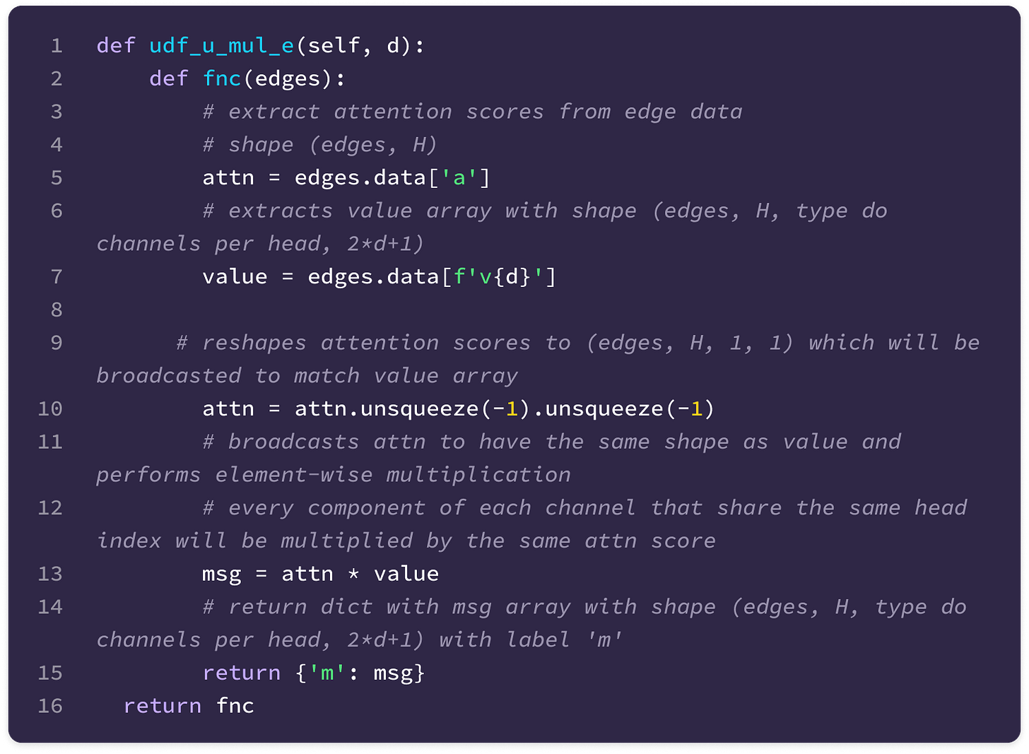
Finally, for every output degree l, we (1) take the sum over the weighted value messages at each attention head and then (2) take the sum over every incoming edge to generate the complete type-l neighbor-to-center message:
\(\mathbf{f}^l_{\text{out},i}=\underbrace{\sum_{j\neq i}^n\underbrace{\sum_{h=1}^H\alpha_{ij,h}\mathbf{v}^l_{ij,h}}_{\text{(1) sum over heads}}}_{\text{(2) sum over all adjacent nodes}}\)The code below loops through all the output degrees, scales the output value messages from the same udf_u_mul_e function as the key embedding, takes the sum of the messages across all attention heads and incoming edges, and finally updates the node features with the aggregated messages.
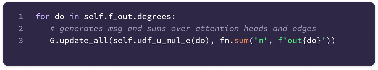
We also return a dictionary where the keys correspond to the output degrees and the values are arrays with shape (nodes, type-l channels, 2l+1) to use for attentive self-interaction:
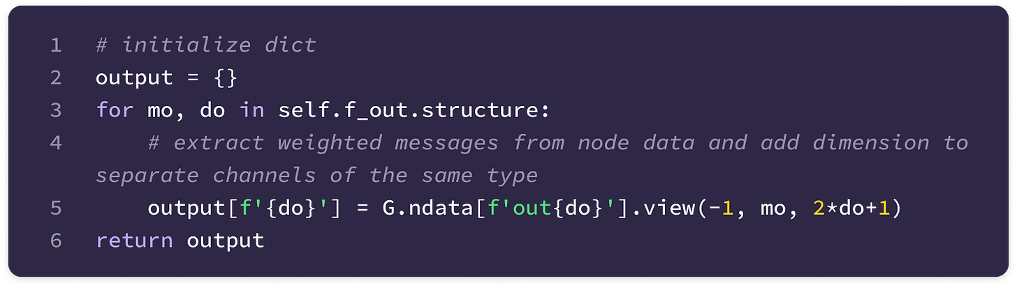
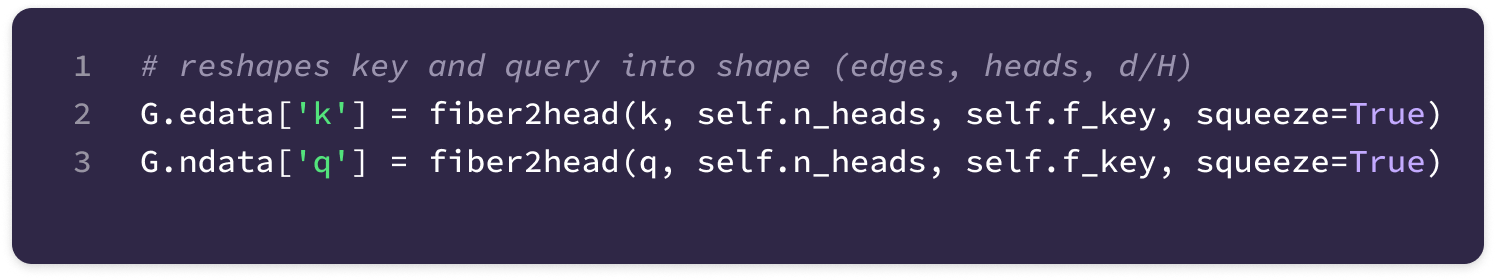
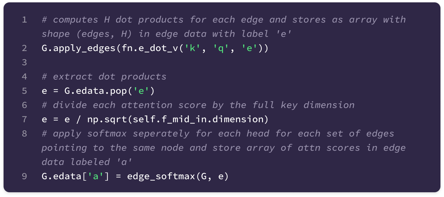
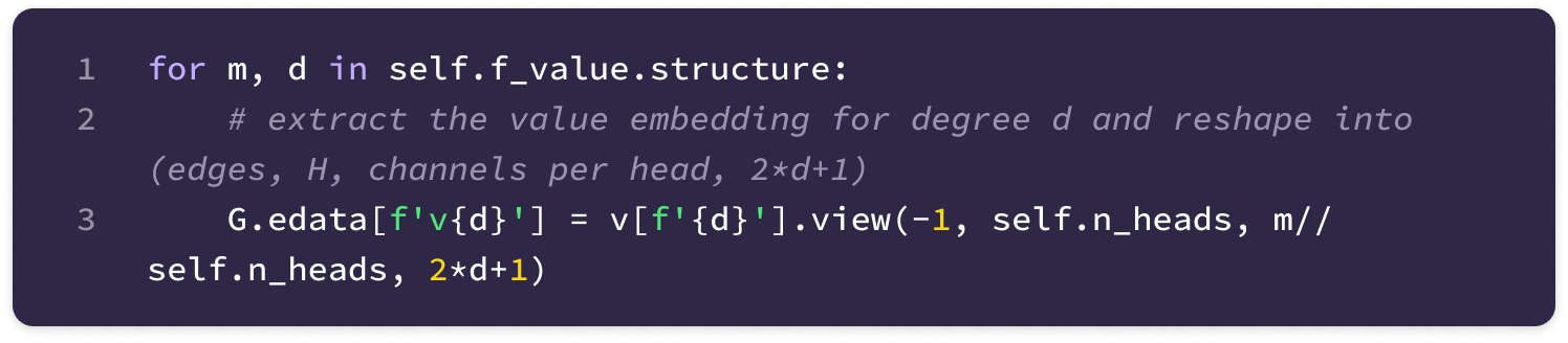
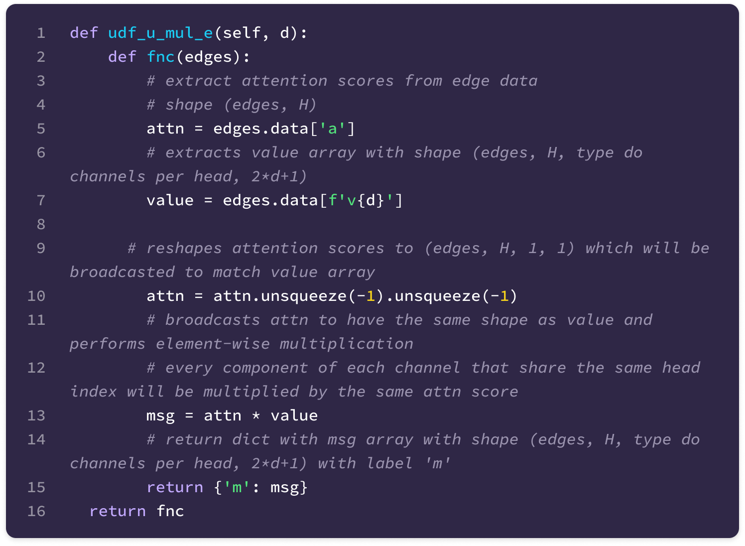
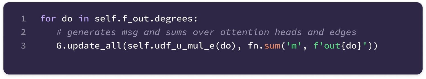
Now, let’s discuss how to incorporate a skip connection and project the value messages to match the output fiber using attentive self-interaction.
Attentive Self-Interaction
The SE(3)-Transformer paper introduced the attentive self-interaction layer which generates self-interaction weights by taking the dot product between pairs of type-l input features and value messages and feeding these raw attention scores into a feed-forward network. Every type-l output channel is a weighted sum of every type-l input channel and every type-l value message scaled by a set of attention scores, capturing patterns across input features from the center node itself and neighbor-to-center messages to generate the output feature tensor.
Attentive self-interaction is a mix of linear self-interaction and channel mixing as it takes a weighted sum of all input channels and all value message channels of the same type to generate the final output tensor, repeating for every output channel with a unique set of attention scores. But instead of initializing the weights randomly and sharing weights across nodes, attentive self-interaction leverages the attention mechanism to compute unique weights for each node and each input-to-output channel pair.
Before generating the attention weights, we take the saved input features of node i before any updates are made and concatenate them to the output of the multi-head self-attention layer. To do this, we define a class GCat that concatenates all the type-l channels in the input fiber to the type-l channels of the value message for every feature type. We can define an instance variable in the constructor of GCat called f_cat that is a fiber object with the same structure as the fiber of value messages f_mid_out added to the multiplicities of the fiber of input features f_in:
The forward function of GCat concatenates the input features to the value messages for all degrees in f_in and returns the concatenated feature tensor in a dictionary called out, where each degree is a label linked to a feature array with shape (nodes, mcat, 2l+1), where mcat denotes the total number of type-l channels in the concatenated tensor.
Now, we can use the concatenated dictionary of features to compute attentive self-interaction and project the concatenated feature tensor to match the structure of the output fiber of the attention layer, f_out. The attentive self-interaction layer generates the type-l output feature at channel c_l as the weighted sum of all the type-l channels in the concatenated fiber with the equation below:
where c_l’ are the indexes of the type-l features in the concatenated fiber and c_l denotes the output type-l channel to which the weighted sum is passed.
Let’s break down the steps to generating the attentive self-interaction term for all the type-l output channels for node i.
First, we generate the set of raw attention scores by taking the dot product of every pair of type-l channels c_l and c_l’ in the concatenated tensor. Since mcat denotes the total number of type-l input channels, a total of mcat*mcat raw attention scores will be generated for the type-l features that can be assembled into a (mcat*mcat)-dimensional vector.
To implement this in code, we loop through every degree and corresponding feature array with shape (mcat, 2l+1) stored in the dictionary. At each iteration, we use PyTorch’s einsum function to calculate the sum of the element-wise product along the last dimension (dot product) for every pair of type-l features along the second last dimension of the type-l feature array, generating an mcat x mcat matrix of raw attention scores.
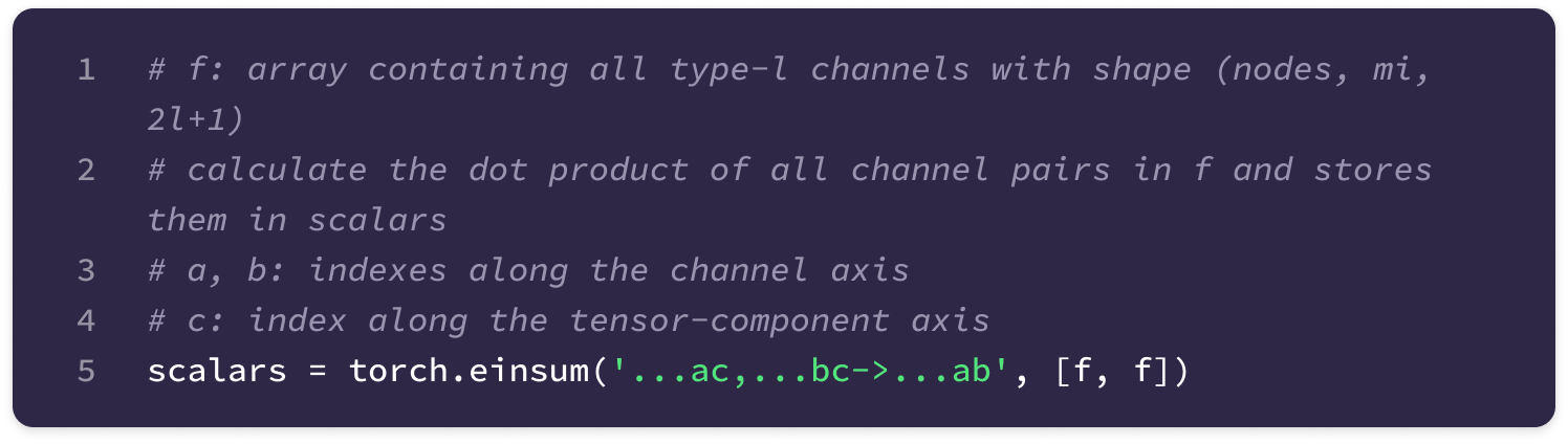
Then, we flatten the scores into a (mcat*mcat)-dimensional vector and ensure that the absolute value of each score is greater than a small constant (1e-12) to avoid vanishing gradients.
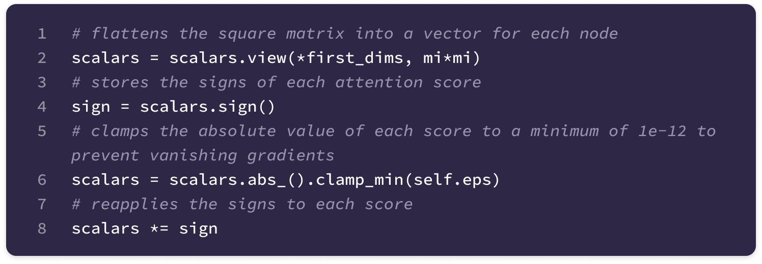
Since the number of output channels (mo) is not always equal to the number of concatenated channels, we need to generate a total of mcat*mo weights for every degree l such that each type-l output channel has a set of mcat weights that are used to calculate a weighted sum of all the type-l input features and value messages.
To convert the (mcat*mcat)-dimensional vector into a (mcat*mo)-dimensional vector of weights, we construct a feed-forward network (FFN) for each feature type with the following layers:
A layer normalization operation that transforms the vector of attention scores to have a mean of 0 and a variance of 1.
A leaky ReLU non-linear activation function is applied element-wise to each attention score. Leaky ReLU is a form of ReLU where, instead of converting all negative inputs to 0, it scales negative inputs by a small integer a to ensure that the gradient exists even for negative inputs. This prevents vanishing gradients caused by negative bias terms in the linear layer.
\(\text{LeakyReLU}(x)=\max(ax, x)\)
Comparison between the ReLU function that returns max(0, x) and the leaky ReLU function that returns max(ax, x). The small constant a ensures that negative values have a non-zero slope to ensure every neuron contributes to gradient descent (Source) A linear layer that transforms the (mcat*mcat)-dimensional vector into a (mcat*mo)-dimensional vector by matrix-vector multiplication with a (mcat*mo) x (mcat*mcat) matrix of learnable weights and addition of a (mcat*mo)-dimensional bias vector. The weights for the linear layer are initialized with the Kaiming initialization, which samples random weights from a uniform distribution U(-bound, bound) with bounds defined by the following equation:
\(\text{bound}=\sqrt{\frac{6}{\text{mcat}\cdot\text{mcat}}}\)This initialization technique is designed specifically for layers using the ReLU or leaky ReLU function to prevent exploding or vanishing gradients by initializing weights such that the variance of the output is approximately equal to the variance of the input. The bias vector is initialized to the zero vector.
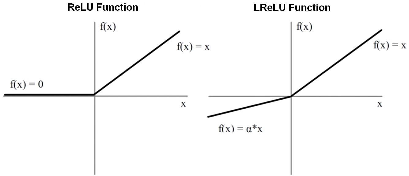
We can construct the FNN for each feature degree by calling the function below:
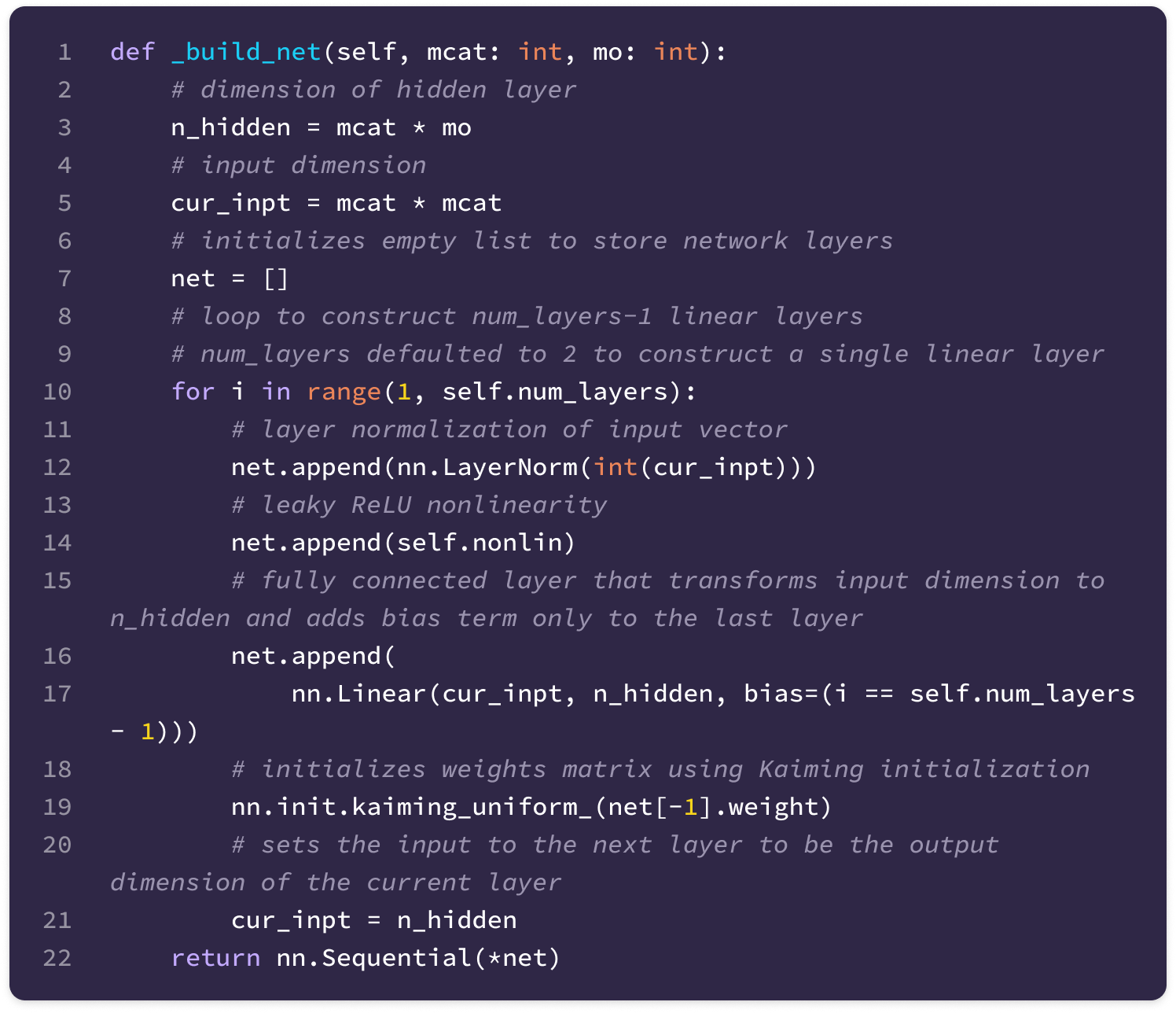
We then loop through all the degrees in the concatenated fiber and use the function above to initialize the FFN with the hidden layer dimension set to the mcat*mo:
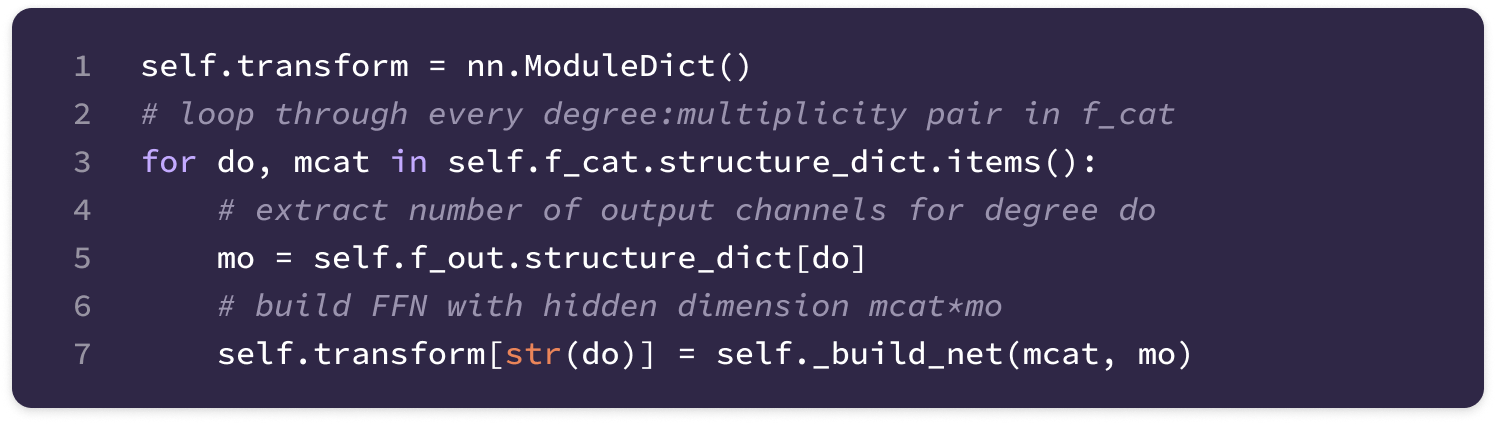
Then, the flattened vector of raw attention scores for degree l is fed into the unique type-l FFN to generate an updated set of mcat*mo attention scores with added dependence on learnable parameters and nonlinearities. This vector is reshaped into a mo x mcat matrix, where each row corresponds to the set of attention scores used to compute self-interaction for a single type-l output channel.
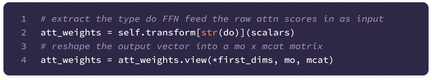
We can now apply the softmax function separately to each row of the attention score matrix (along the last dimension) such that the scores of each row add up to 1. This normalizes the set of weights used to scale all the concatenated channels for a single type-l output channel into probabilities that sum to 1.
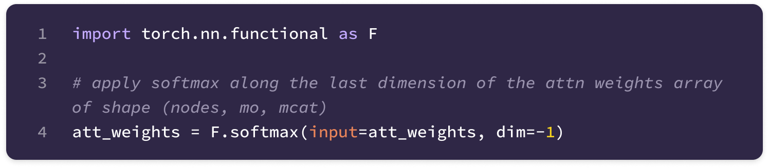
Finally, we can generate a self-interaction message for each output channel c_l with the weighted sum of every type-l input feature and value message scaled by their attention score. The attention scores measure the similarity of the channel feature to all the other channels of the same type, which produces a self-interaction message that effectively captures patterns from both the input features of the node itself and the value messages from neighboring nodes.
This step is performed in parallel for every output channel of a single degree via matrix-matrix multiplication between the mo x mcat matrix of attention weights and the mcat x (2l+1) matrix of type-l features in the concatenated feature array.
The matrix multiplication can be implemented using the einsum function that takes the sum of the element-wise products of the elements along the columns of the attention matrix with the elements along the rows of the feature matrix to produce a (mo, 2l+1) array of self-interaction messages for every type-l output channel.
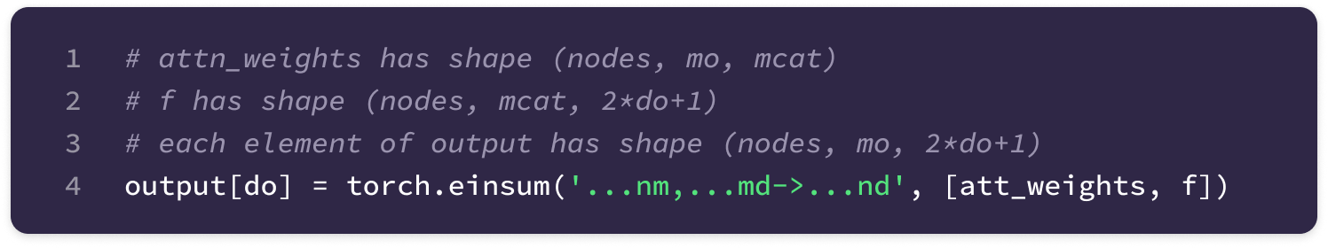
Finally, we can update the feature tensor at node i with the attentive self-interaction messages that match the output fiber structure, f_out:
The purpose of the attentive self-interaction is four-fold:
In the sequence-based Transformer model, every element in the sequence attends to all other elements, including itself. Since the neighbor-to-center message does not include features from the center node, attentive self-interaction introduces a way for the node to attend to its own features, allowing the model to learn the contributions of the features of a single atom or molecular unit to the prediction task.
Unlike linear self-interaction and channel-mixing, which use a single weight for each feature channel shared across all nodes, attentive self-interaction generates unique weights for each node to produce self-interaction messages that reflect the contextual patterns across input features and value messages of each node.
The attention scores place additional weight on features that are similar to the other features of the same type to ensure that a cohesive set of output features is used to update the center node.
Since the value messages primarily carry information from neighborhood nodes and edges, concatenating the input features to the value messages introduces a skip connection that ensures that the original node information is not lost. The attention weights process the concatenated features with learnable parameters to determine the relative importance of each piece of information. The skip connection also allows the gradient to skip past the potentially gradient-diminishing message-calculation transformations during backpropagation to avoid vanishing gradients.
Furthermore, the attentive self-interaction weights and the weighted sum operation satisfy the rules for equivariant layers defined above.
Now that we have defined all the components of the attention block, we can initialize all the relevant module objects in the constructor of the GSE3Res module:
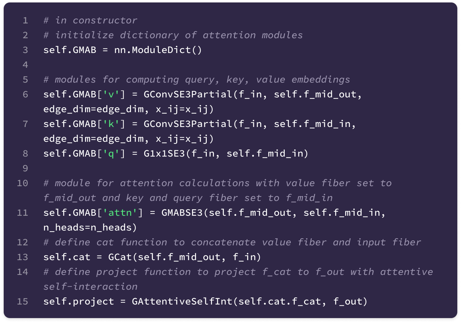
In the forward pass, these functions are called in the following order to generate the updated feature tensors for every node in the graph:
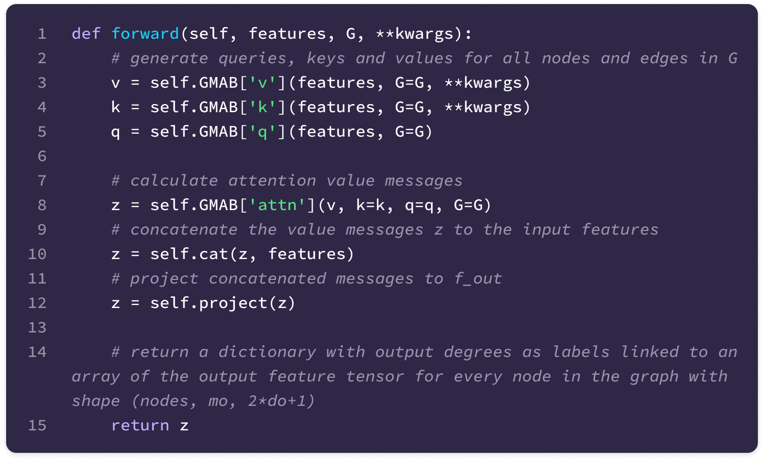
Norm Nonlinearity
Following each attention block, the SE(3)-Transformer incorporates a SE(3)-equivariant ReLU normalization and nonlinearity module with a feed-forward network. This module stabilizes the distribution of features across layers for smoother gradient flow and adds an extra degree of nonlinearity to the attention block without breaking equivariance.
The norm nonlinearity layer is applied to each feature type separately. The following steps are performed on all type-l output features in a single node in the graph:
The Euclidean norm (L2 norm) is applied across all type-l features, which calculates the magnitude (or length) of each type-l feature vector in (2l+1)-dimensional Euclidean space. All the norms of the type-l feature channels are stored in a single mo-dimensional vector, where mo denotes the number of type-l channels in the output fiber of the attention block. The norm for a single type-l channel is given by the equation below, where the double-bar and subscript denote the L2 norm:
\(||\mathbf{f}^l_{c_l}||_2=\sqrt{\sum_{m=-l}^l(f^l_m)^2}\)The following code generates an array with shape (mo, 2l+1) where all the elements along the c_lth row are equal to the norm corresponding to the channel c_l, in preparation for element-wise division.
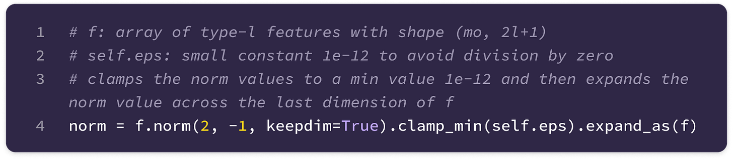
Then, each type-l feature is divided element-wise by the corresponding norm to generate a unit-length vector in the direction of the feature (similar to generating the angular component of the displacement vector).
\(\frac{\mathbf{f}_{c_l}^l}{||\mathbf{f}_{c_l}^l||_2}=\begin{bmatrix}\frac{f^l_{-l}}{||\mathbf{f}_{c_l}^l||_2}\\\vdots\\\frac{f^l_l}{||\mathbf{f}_{c_l}^l||_2}\end{bmatrix}\)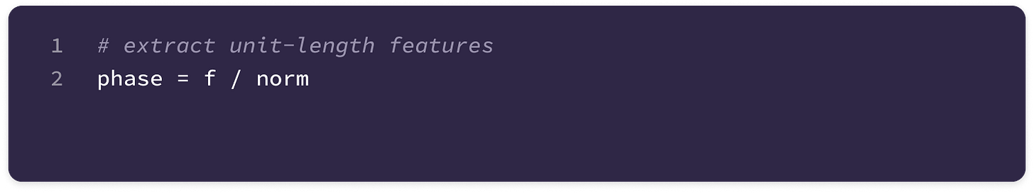
To incorporate learnability and nonlinearity to the normalization of type-l output, we construct an FFN that takes the norms across all type-l output channels and applies the following operations (1) a layer normalization step that shifts the mean to 0 and variance to 1 across all type-l norms, (2) a ReLU nonlinearity that converts all negative norms from step 1 to 0 while keeping all positive norms the same and (3) an (optional) linear layer that transforms the norms without changing the dimension through matrix multiplication with learnable weights and addition of a bias vector.
\(\text{FFN}(||\mathbf{f}^l||_2)=\underbrace{\mathbf{W}_{(\text{mo}\times\text{mo)}}\underbrace{\max\left(0,\text{LayerNorm}(\underbrace{\bigoplus_{c_l}||\mathbf{f}^l_{c_l}||_2}_{\text{all type-}l\text{ norms}})\right)}_{\text{ReLU nonlinearity}}+\mathbf{b}}_{\text{linear layer}}\)This FFN can be built by calling the function below:

We call the function above in a loop to construct a unique FFN for every feature type:
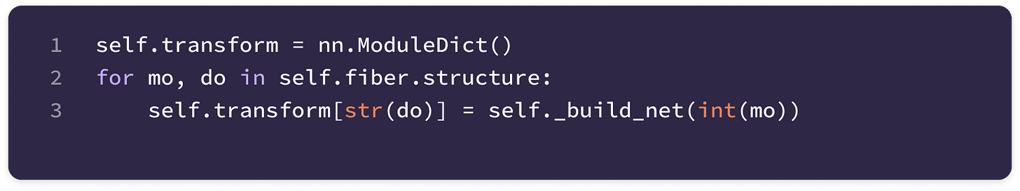
Next, we call the transform function on the mo-dimensional vector of norms, which generates a weight for each type-l channel. Then, we add a singleton dimension that will be broadcasted for element-wise multiplication in the next step.
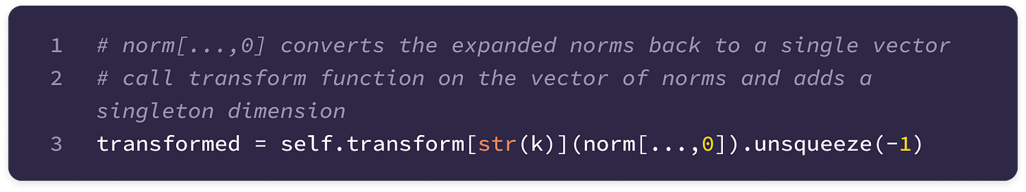
Finally, we scale each type-l channel divided by its L2 norm with the corresponding nonlinear weight generated from the FFN to get the final normalized feature at channel c_l.
\(\text{NormNonlinear}(\mathbf{f}^l_{c_l})=\text{FFN}(||\mathbf{f}^l||_2)_{c_l}\begin{bmatrix}\frac{f^l_{-l}}{||\mathbf{f}_{c_l}^l||_2}\\\vdots\\\frac{f^l_l}{||\mathbf{f}_{c_l}^l||_2}\end{bmatrix}\)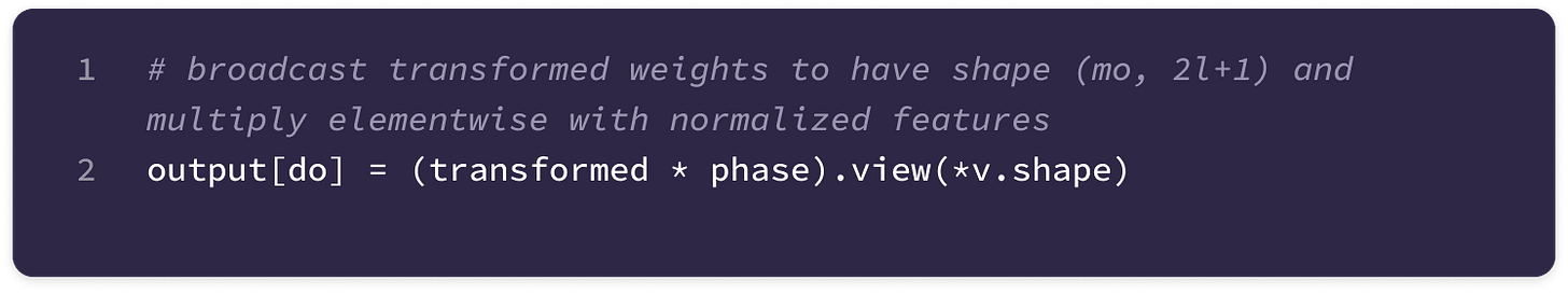
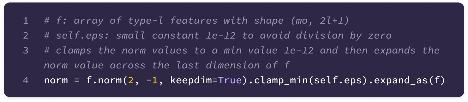
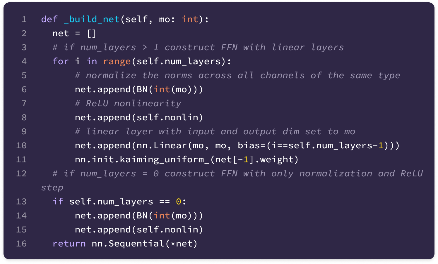
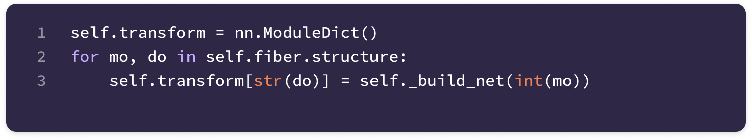
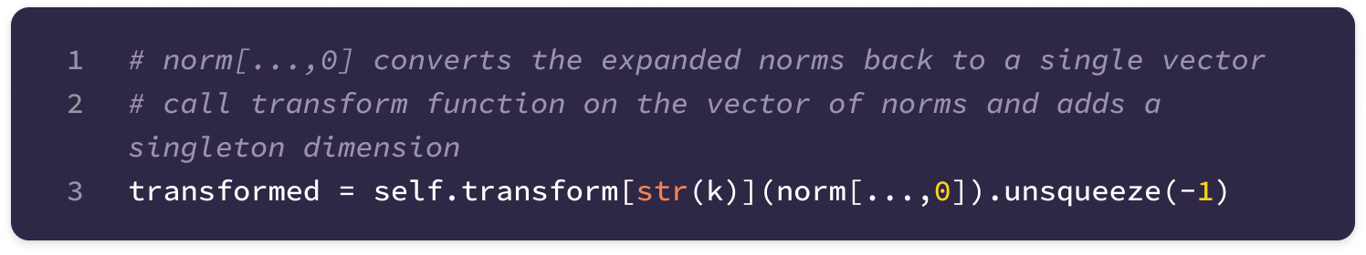
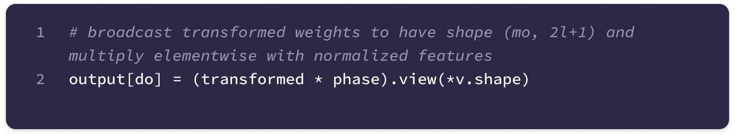
Incorporating Edge Features
Edge features can store both information on the interaction between nodes and the nodes themselves. Previously, we discussed how to incorporate the angular unit displacement vector (type-1 edge feature) and radial distance (type-0 edge feature) via learnable functions that allow the model to learn dependencies on the spatial positioning of nodes.
Graphs can also contain other edge features (e.g., bond type, shared electrons, etc.) that can be incorporated into equivariant message-passing layers in the following ways:
If the edge feature is a scalar (type-0 tensor), it can be used to scale basis kernels during kernel construction, similar to the radial functions. This can be done by extending the learnable radial FFN to take multiple scalars (in the form of a vector) as input. This would allow the radial network to learn dependencies between the radial distance and additional scalar edge features and produce kernel weights dependent on these additional edge features.
\(\begin{align}\mathbf{W}^{lk}(\mathbf{x}_{ij})=\sum_{J=|k-l|}^{k+l}\varphi^{lk}_J(||\mathbf{x}_{ij}||, \mathbf{f}_{ij}^{(0)})\mathbf{W}^{lk}_J(\mathbf{x}_{ij})\tag{$\mathbf{f}_{ij}^{(0)}\in \mathbb{R}$}\end{align}\)The function denoted by phi takes two type-0 spherical tensors, including radial distance, and converts them into a scalar weight:
\(\varphi^{lk}_J:\mathbb{R}^2\to\mathbb{R}\)The code below concatenates type-0 edge features to the radial distance and feeds the vector of type-0 features into the radial network to generate the unique set of weights used to scale the basis kernels:
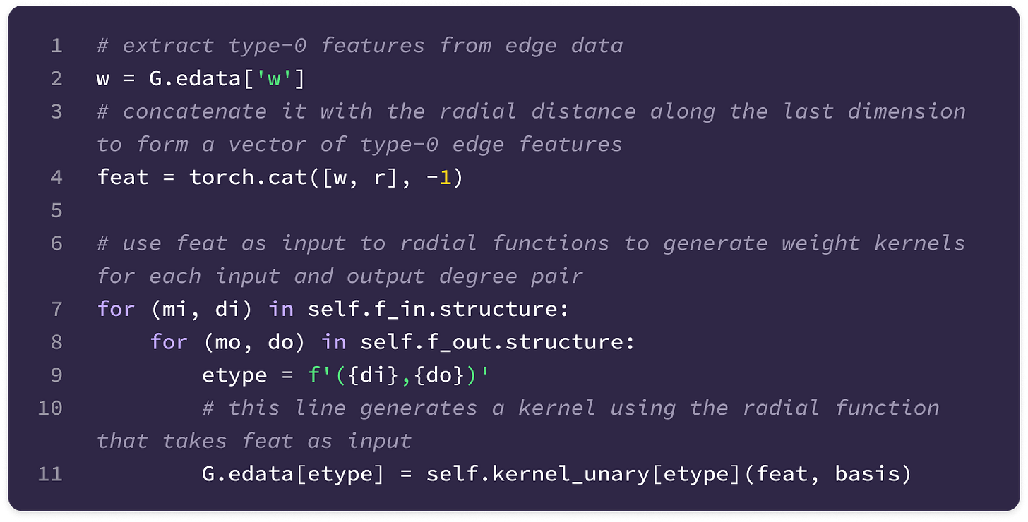
An alternative way to incorporate scalar edge features is to construct separate learnable FFNs specifically trained to learn dependencies on the specific edge feature, producing a scalar weight that is used in conjunction with the radial weight to scale the basis kernels.
\(\begin{align}\mathbf{W}^{lk}(\mathbf{x}_{ij})=\sum_{J=|k-l|}^{k+l}\psi^{lk}_J(\mathbf{f}_{ij}^{(0)})\varphi^{lk}_J(||\mathbf{x}_{ij}||)\mathbf{W}^{lk}_J(\mathbf{x}_{ij})\tag{$\mathbf{f}_{ij}^{(0)}\in \mathbb{R}$}\end{align}\)Psi (ψ) denotes the FFN that takes a scalar edge feature to a set of (2min(l, k)+1)*(input channels)*(output channels) weights used to scale each basis kernel for every pair of input and output channels:
\(\psi^{lk}(\mathbf{f}_{ij}^{(0)}):\mathbb{R}\to\mathbb{R}^{(2min(l,k)+1)(\text{mi})(\text{mo})} \)Higher-degree (k >= 1) edge features can be transformed from type-k to type-l tensors via equivariant kernels and then used in the self-attention mechanism just like the node features. This is done by concatenating the edge features to the features of the source node of the same type just before they are transformed into type-l key embeddings for computing attention weights and value embeddings for computing the neighbor-to-center messages.
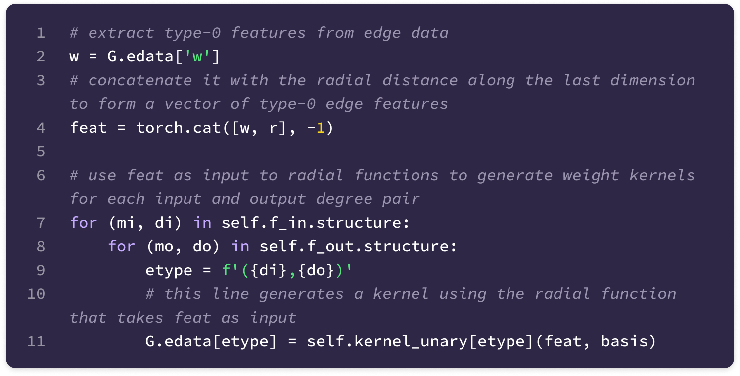
To incorporate edge features, the SE(3)-Transformer module concatenates the full relative displacement vector (as opposed to the unit displacement vector used as input to spherical harmonics) as a type-1 edge feature with the type-1 node features before calculating the key and value embeddings.
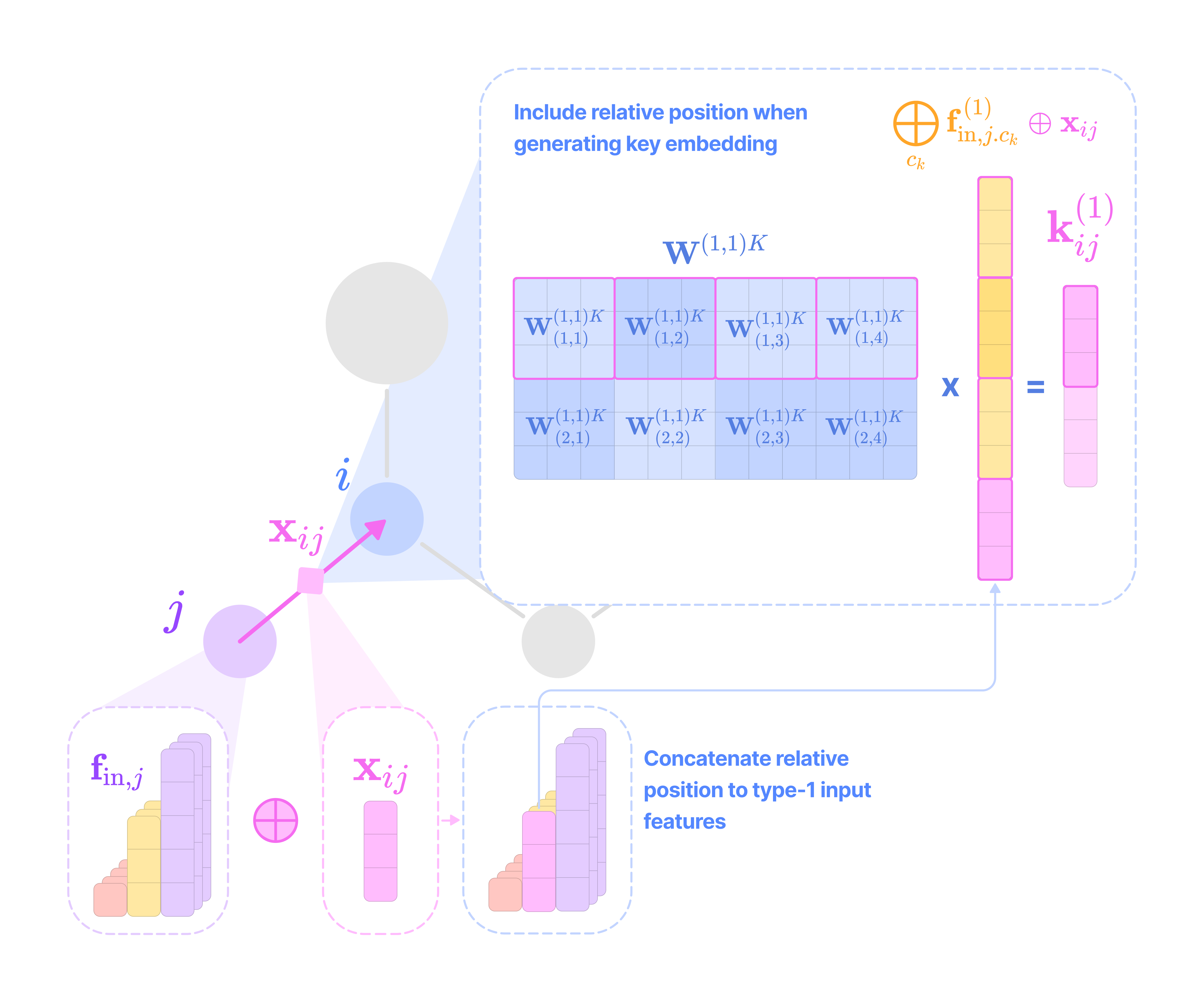
First, the multiplicity for degree 1 in the input fiber is incremented by 1 if the displacement is concatenated (multiplicity is unchanged for addition).
Now, we can incorporate the type-1 displacement vector stored in the edge either through concatenation or addition to the type-1 input features before multiplying with the key and value kernels and generating the key and value embeddings:
Chemical Property Prediction
The SE(3)-Transformer model was tested on the QM9 dataset of 134K small molecules for the prediction of system-level chemical properties that are invariant to translations and rotations in 3-dimensions.
The model performance was evaluated for the prediction of six chemical properties including α (isotropic polarizability), ϵ_HOMO (energy of the highest occupied molecular orbital), ϵ_LUMO (energy of the lowest unoccupied molecular orbital), Δϵ (energy gap which equals LUMO - HOMO), μ (dipole moment), and Cv (heat capacity at constant volume). These are regression tasks as the values for the different properties are continuous.
The diagram below shows the full architecture used on the QM9 dataset:
Initializing the Graph
Each node of the graph represents an atom in the molecule, with up to a maximum of 29 atoms or nodes in a graph. Each node embeds a 6-dimensional vector for the following features:
The atomic species (Hydrogen, Carbon, Oxygen, Nitrogen, or Fluorine) is represented as a 5-dimensional one-hot-embedding vector with a 1 corresponding to the species of the node and zeros everywhere else.
The atomic number or number of protons in the atom is represented as a scalar integer value.
All node features are type-0 tensors, so there are a total of 6 type-0 channels in the initial node feature tensor.
The graph is a sparse molecular graph where only the bonded atoms are connected by a bidirectional edge, meaning the nodes at either end of the edge can send and receive messages to each other. Each edge embeds a 5-dimensional vector storing the following features:
The type of chemical bond (single, double, triple, or aromatic bond) is represented as a 4-dimensional one-hot encoding vector corresponding to the bond type between the nodes that it connects.
The Euclidean distance between atoms is represented as a scalar.
All edge features are also type-0 tensors, so there are a total of 5 type-0 channels in the initial feature tensor corresponding to each edge.
The code below initializes the DGL graph using two arrays storing the source and destination node indices that are aligned such that a position i in the source array and the destination array corresponds to a single edge in the graph. Then, the node and edge features are stored as arrays that can be accessed with the corresponding label.
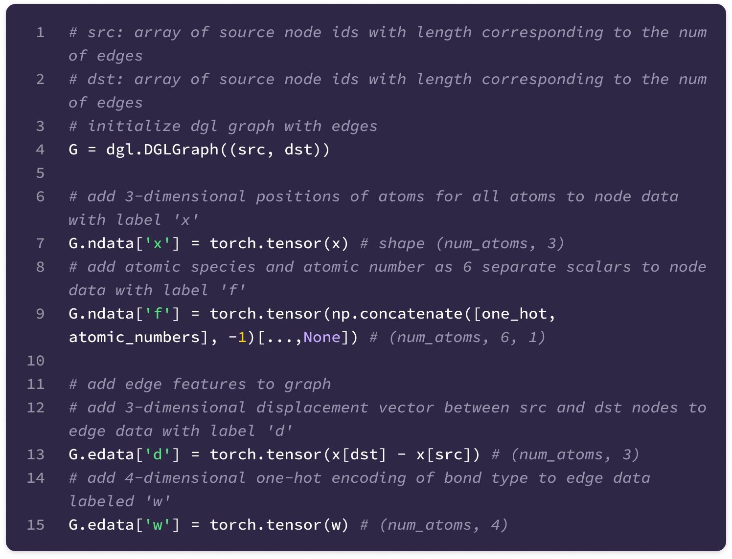
Encoder
The encoder consists of 7 multi-head (H=8) attention blocks each of which is followed by an equivariant norm nonlinearity layer. The first attention block converts the 6 channels of type-0 node features into type-0, type-1, type-2, and type-3 feature channels with 32 channels each. This is followed by 6 identical blocks that computes 16 channels for each type of value message and projects it back to 32 channels using attentive self-interaction. The output is a learned internal representation for each feature channel of each atom that encodes dependencies between bonded atoms.
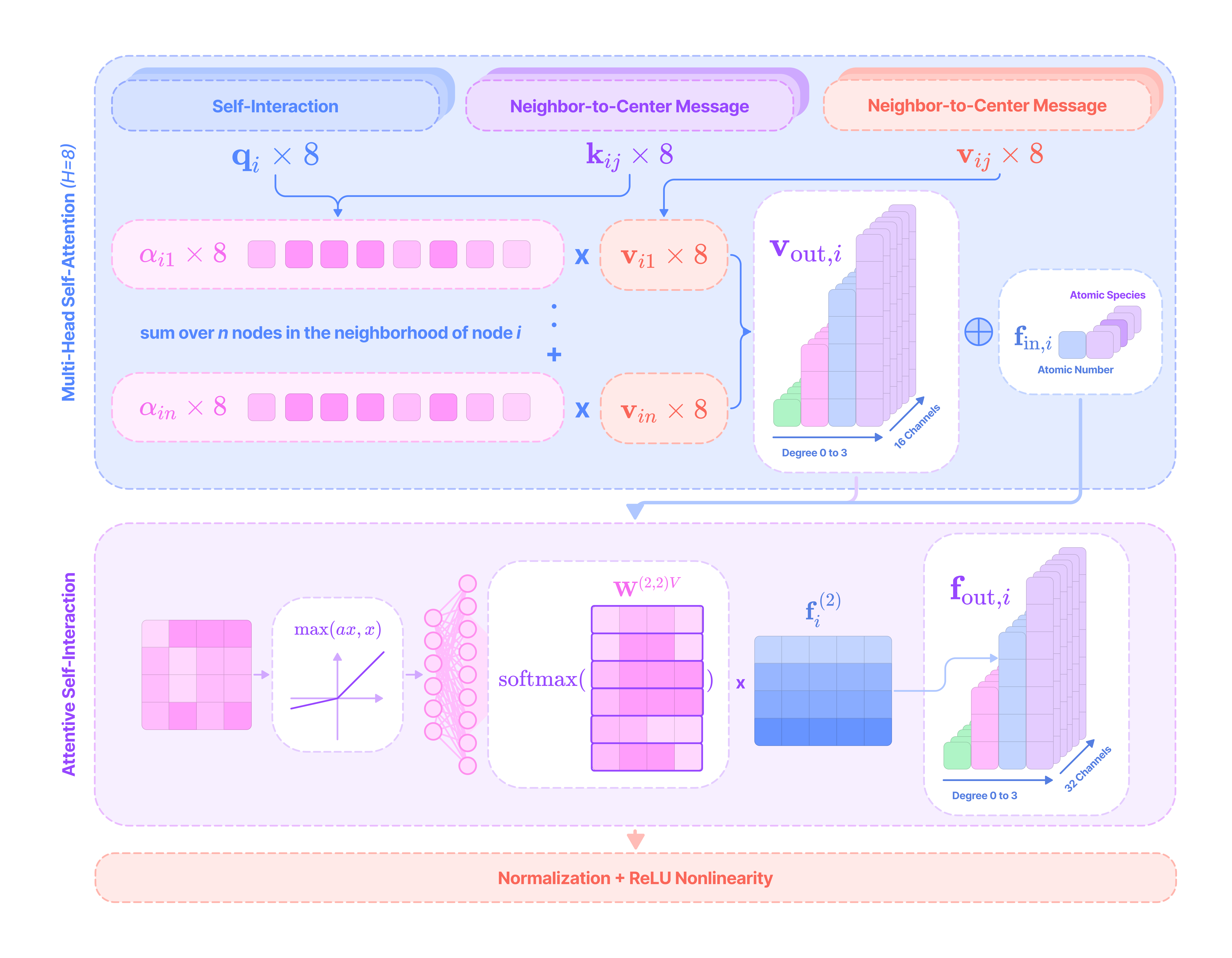
The encoder is composed of 7 multi-head attention blocks, each with 8 attention heads.
The first attention block takes six channels of type-0 features as input and outputs a feature tensor with type-0, type-1, type-2, and type-3 spherical tensors, each with 32 channels for every node in the graph. The input, key/query (f_mid_in), value (f_mid_out), and output fibers are defined below:
f_in = [(input channels, input degree)] = [(4, 0)]
f_mid_in = [(16, 0)]
f_mid_out = [(16, 0), (16, 1), (16, 2), (16, 3)]
f_cat = [(20, 0), (16, 1), (16, 2), (16, 3)]
f_out = [(output channels, output degrees)]= [(32, 0), (32, 1), (32, 2), (32, 3)]
This block generates 16 channels of value messages for each output degree before concatenating with the input type-0 features and projecting it to match the output fiber f_out using attentive self-interaction.
Since the graph contains multiple type-0 scalar edge features in addition to the radial distance, the model concatenates them into a single 5-dimensional vector, where the first dimension corresponds to the radial distance and the remaining four dimensions correspond to the one-hot encoding of the bond type. Instead of just the radial distance, this 5-dimensional vector is fed into the radial function to generate the weights used to scale the basis kernels.
The first attention block executes the multi-head self-attention layer as follows:
Since the query embeddings are generated via self-interaction, we can only compute type-0 query embeddings from the type-0 input features. For each edge, we generate 16 query embeddings, each of which is a linear combination of the input type-0 channels. Then, we split them into 8 attention heads and concatenate the two embeddings at each head into a single 2-dimensional vector to get a query array with shape (edges, 8, 2).
The key embeddings must have the same dimension as the query embedding so we only generate key embeddings for degree 0 with shape (edges, 8, 2). For each edge, we generate 16 key embeddings by transforming the four channels of type-0 input tensors to 16 channels of type-0 key embeddings using 4*16 = 64 unique 1 x 1 (scalar) key kernels corresponding to each input and output channel pair. Then, we split them into 8 attention heads and concatenate the two embeddings at each head into a single 2-dimensional vector.
For each edge, 8 unique attention weights are generated from the dot product of the query and key vectors for the 8 attention heads, each of which scales a total of 8 value embeddings (2 for each output degree).
The value array corresponding to each output degree has shape (edges, 8 (heads), 2 (channels per head), 2l + 1) for l = 0, 1, 2, 3. For each edge and each output degree l, the 4 type-0 input channels are transformed into 16 channels of type-l value embeddings using 4*16 = 64 unique (2l+1) x 1 value kernels corresponding to each input and output channel pair. These value embeddings are then divided into 8 attention heads with 2 channels per degree per head.
Every channel of every node in the graph is updated with the weighted sum of the value embeddings from incoming edges.
The first attention block is followed by six identical attention blocks with the same input and output fiber. The intermediate value fiber divides the channels in half before projecting them to match the output fiber using attentive self-interaction. The fiber structures for all six attention blocks are defined below:
f_in = [(32, 0), (32, 1), (32, 2), (32, 3)]
f_mid_in = [(16, 0), (16, 1), (16, 2), (16, 3)]
f_mid_out = [(16, 0), (16, 1), (16, 2), (16, 3)]
f_cat = [(48, 0), (48, 1), (48, 2), (48, 3)]
f_out = [(32, 0), (32, 1), (32, 2), (32, 3)]
There are some key differences from the first attention block given the higher dimension of the input features:
The value array for each degree has the same shape as the first attention block. Since there are 4*16 = 64 input channels and 64 output channels across all degrees, there are a total of 64² unique value kernels for each input-output channel/degree pair.
Instead of only type-0 query embeddings, 16 query embeddings of each type from 0 to 4 are generated from the self-interaction of the input features. These are split into heads and concatenated into a single vector per head, such that the query array has shape (edges, 8, dimension of query/8).
The key embedding for a given channel of a given degree in the center node is generated by aggregating transformed messages from every channel of every degree in the source node. Just like the query embedding, they are split into heads and concatenated into an array with shape (edges, 8, dimension of query/8).
Each attention block is followed by a norm nonlinearity layer described earlier that normalizes across all the features of the same degree for every node in the graph and incorporates the ReLU nonlinearity. The output of the final attention block is a fiber with structure [(32, 0), (32, 1), (32, 2), (32, 3)] that is fed into the decoder.
Decoder
The decoder consists of a TFN module that transforms the high-dimensional features back down to a total of 128 type-0 feature channels. These are scalars invariant to rotation, so they can be passed into a FFN to generate the final prediction.
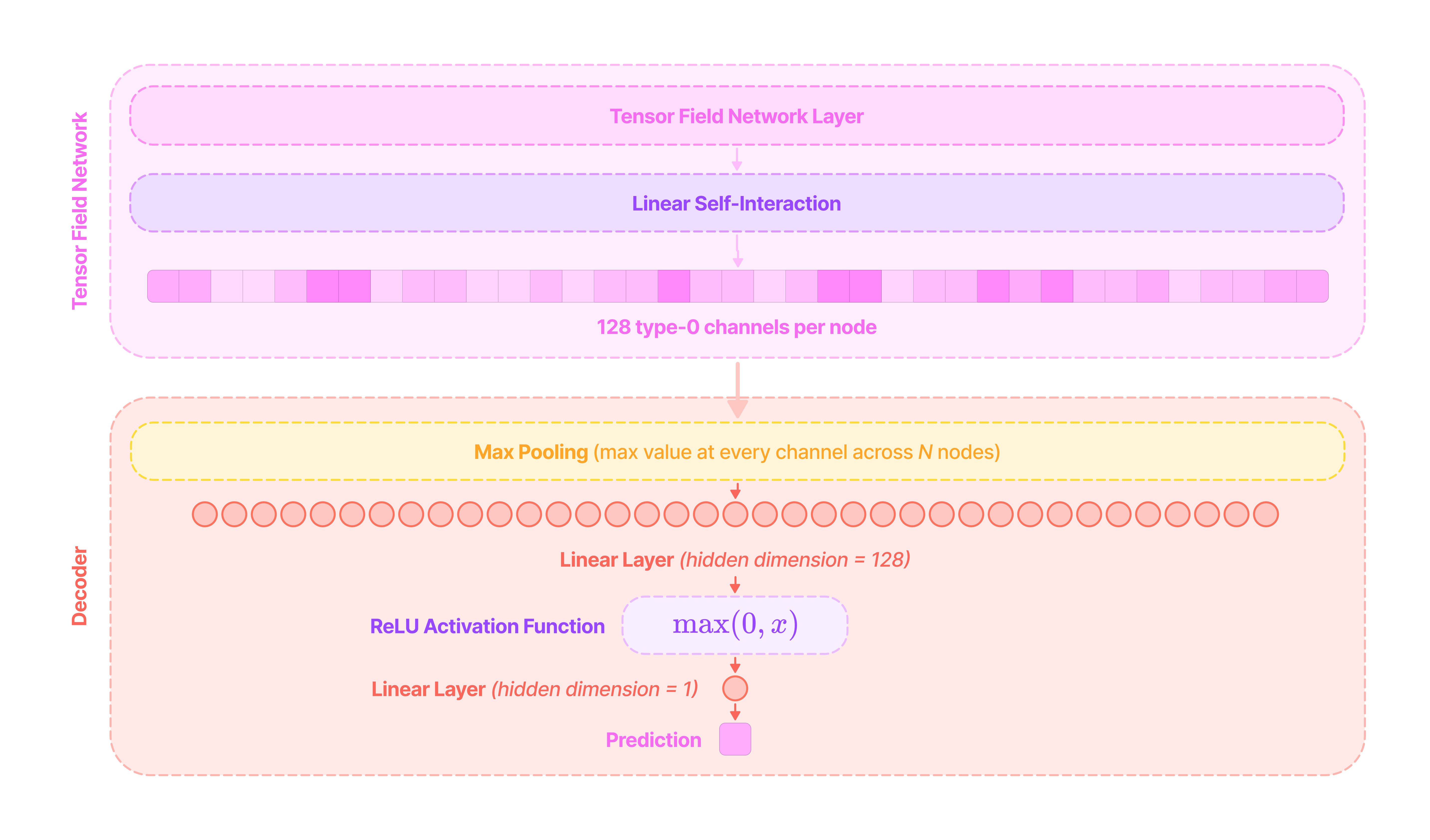
The first block of the decoder is a TFN layer that converts the fiber with structure [(32, 0), (32, 1), (32, 2), (32, 3)] to a fiber with structure [(128, 0)].
Each type-0 output channel of the TFN layer is generated by adding a neighbor-to-center message with a linear self-interaction message.
For each edge, there are 128 total input channels across all degrees and 128 type-0 output channels, so the TFN layer uses a total of 128² unique 1 x (2k+1) equivariant kernels that transform from type-k input channels for k = 0, …, 3 to type-0 output channels. The neighbor-to-center message for a single node is the average of the type-0 messages across all incoming edges.
A linear self-interaction message is computed for all 128 type-0 output channels as a weighted sum of the 32 type-0 input channels. This type-0 message is added to the neighbor-to-center message and acts as a skip connection in gradient descent.
The output of the TFN module is a graph with a 128-dimensional vector at every node, where each element of the vector is a type-0 scalar invariant to rotation. This means that we can apply any function to these vectors without breaking the equivariance of the model.
The resulting graph is fed into a max pooling layer that reduces the feature data across all nodes into a single set of 128 type-0 channels by extracting the maximum type-0 scalar at each channel c_k across every node in the graph.
The implementation of the max pooling mechanism for graph inputs is given below:
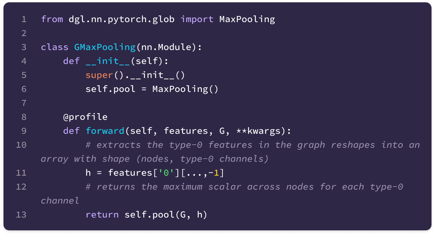
An alternative way to reduce the type-0 feature data across the graph is by using an average pooling layer, where instead of taking the maximum across all nodes, we take the average.
The pooling layer reduces the graph into a single 128-dimensional vector that is fed into an FFN. The first linear layer of the FFN transforms the vector without reducing its dimension with a 128 x 128 learnable weight matrix and 128-dimensional bias vector. Then, a ReLU activation function is applied element-wise to the vector. The final linear layer transforms the 128-dimensional vector into a single scalar prediction with a 128 x 1 weight matrix and a single bias.
Training
The SE(3)-Transformer architecture was trained for 50 iterations (epochs) using the Adam optimizer with a learning rate 1e-3 and a batch size of 32.
Since the chemical properties stored in QM9 are invariant to rotations in SO(3), we need to evaluate whether the model’s predictions change with rotations to the positions of the atoms.
For datasets with node or edge features with degrees greater than 0, both the input coordinates and feature tensors must be rotated to evaluate equivariance. For tasks where the outputs are tensors with degrees greater than 0 (e.g. 3D coordinates, force vectors), the input data and output labels need to be rotated to evaluate equivariance. Since the QM9 dataset only contains type-0 features, equivariance was evaluated by applying random rotations to the coordinate positions across all atoms in a molecule.
The loss or error for each iteration is computed by taking the sum of the absolute differences between the model prediction and the label value across the batch and rescaling the loss from its normalized form to the original scale of the chemical property data.
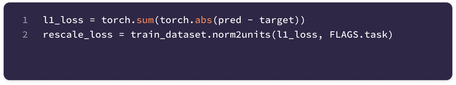
The rescaling function is defined as:
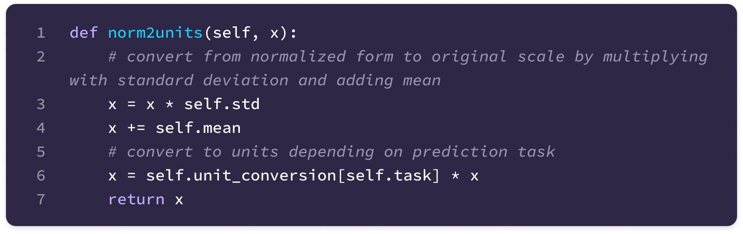
The model uses the Adam optimizer for gradient descent, which adapts the step size (scalar that is multiplied with the learning rate to determine the magnitude of parameter updates) for each epoch and parameter depending on the first and second moments of the gradient, enabling stable updates and faster convergence (see my previous article for a deeper explanation).
The model also gradually decreases the learning rate to a minimum of 1e-4 based on a single-cycle cosine function to prevent overshooting. We can define the Adam optimizer and cosine decay with the following code:
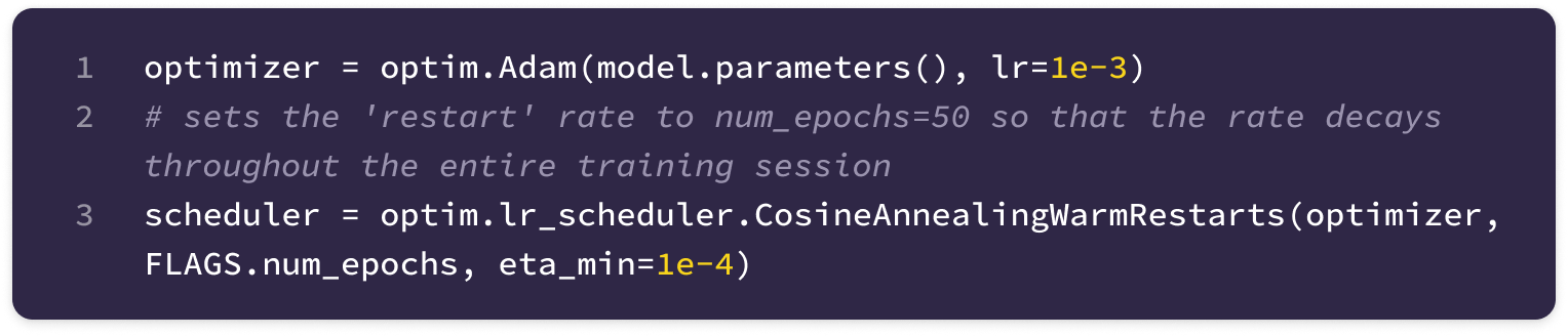
The SE(3)-Transformer architecture showed competitive performance against both non-equivariant and equivariant models. The error of the SE(3)-Transformer was lower for all prediction tasks against the TFN baseline, indicating that the self-attention mechanism increases predictive performance.
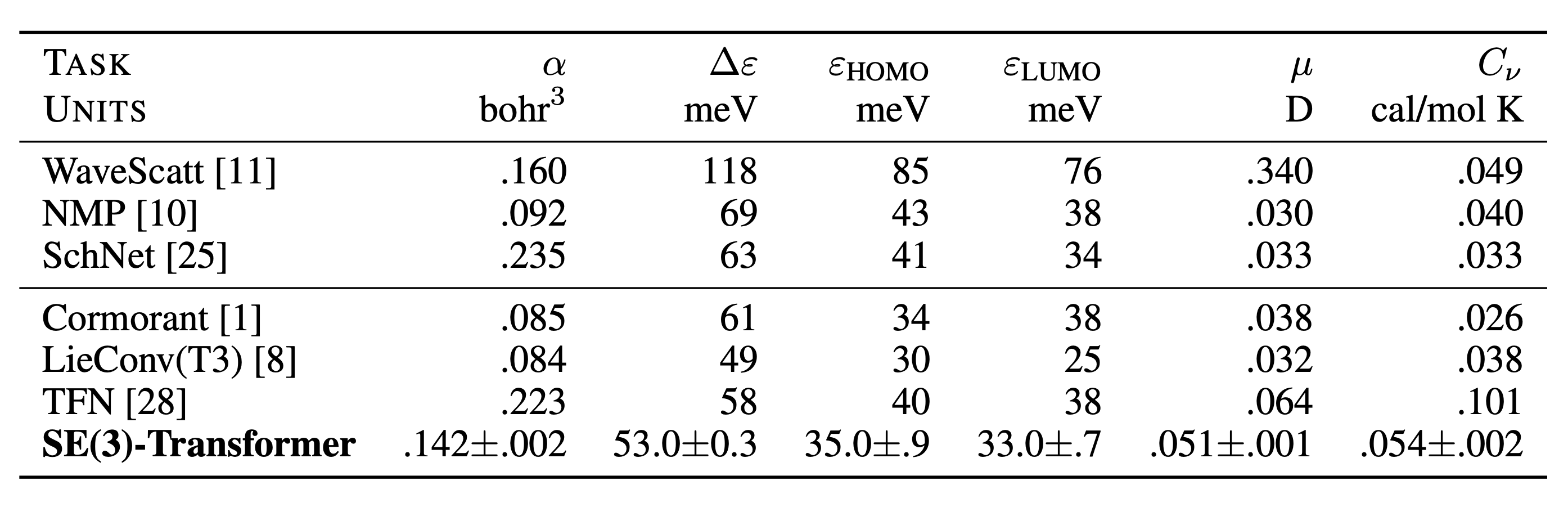
Conclusion
If you’ve made it to the end of this long article, it is likely because you find the applications of deep learning on geometric graph representations of physical systems—especially biomolecules—as fascinating as I do. If so, consider following along in my journey through more deep dives into bio-ML concepts by subscribing.
In an upcoming article, I will be breaking down the RoseTTAFold model that uses SE(3)-Transformer layers in its structure module to refine the positions of C-alpha atoms in the protein backbone as well as the displacement vectors representing peptide bonds. I’m also planning on introducing how to integrate iteration into equivariant geometric GNNs for generative modeling and design of proteins and biomolecules.
Thank you for reading! If you have any suggestions, please feel free to reach out via LinkedIn. Listed below are the journal articles I referenced while writing this article:
Fuchs et al. “SE(3)-Transformers: 3D Roto-Translation Equivariant Attention Networks.” arXiv, November 24, 2020. http://arxiv.org/abs/2006.10503.
Duval et al. “A Hitchhiker’s Guide to Geometric GNNs for 3D Atomic Systems.” arXiv, March 13, 2024. https://doi.org/10.48550/arXiv.2312.07511.
Geiger and Smidt. “E3nn: Euclidean Neural Networks.” arXiv, July 18, 2022. https://doi.org/10.48550/arXiv.2207.09453.
Weiler et al. “3D Steerable CNNs: Learning Rotationally Equivariant Features in Volumetric Data.” arXiv, October 27, 2018. http://arxiv.org/abs/1807.02547.
Bronstein et al. “Geometric Deep Learning: Grids, Groups, Graphs, Geodesics, and Gauges.” arXiv, May 2, 2021. http://arxiv.org/abs/2104.13478.
Cohen et al. “Intertwiners between Induced Representations (with Applications to the Theory of Equivariant Neural Networks).” arXiv, March 30, 2018. http://arxiv.org/abs/1803.10743.
Schütt et al. “SchNet: A Continuous-Filter Convolutional Neural Network for Modeling Quantum Interactions.” arXiv, December 19, 2017. http://arxiv.org/abs/1706.08566.
Thomas et al. “Tensor Field Networks: Rotation- and Translation-Equivariant Neural Networks for 3D Point Clouds.” arXiv, May 18, 2018. https://doi.org/10.48550/arXiv.1802.08219.
Alchemy Bio is a blog where I share transformational ideas in computational biology, synbio, and biotech. If you don’t want to miss upcoming blogs, you should consider subscribing for free to have them delivered to your inbox:
Real spherical harmonics are often used in machine learning applications to reduce computational complexity; however, complex spherical harmonics are used in quantum mechanics.
A function is square-integrable on [-1, 1] if the integral (area under the curve) of the function squared on the domain [-1, 1] is less than infinity (bounded). This is an important property of wavefunctions in quantum mechanics because the square of a wavefunction represents a probability distribution with an integral of 1.